Category: Life Style

The world must rethink plans for ageing oil and gas platforms

Post author By lisa nichols
Post date March 10, 2024
No Comments on The world must rethink plans for ageing oil and gas platforms

[ad_1]

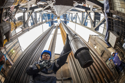
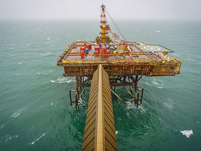
One of world’s largest oil platforms, the North Sea’s Gullfaks C, sits on immense foundations, constructed from 246,000 cubic metres of reinforced concrete, penetrating 22 metres into the sea bed and smothering about 16,000 square metres of sea floor. The platform’s installation in 1989 was a feat of engineering. Now, Gullfaks C has exceeded its expected 30-year lifespan and is due to be decommissioned in 2036. How can this gargantuan structure, and others like it, be taken out of action in a safe, cost-effective and environmentally beneficial way? Solutions are urgently needed.

Many of the world’s 12,000 offshore oil and gas platforms are nearing the end of their lives (see ‘Decommissioning looms’). The average age of the more than 1,500 platforms and installations in the North Sea is 25 years. In the Gulf of Mexico, around 1,500 platforms are more than 30 years old. In the Asia–Pacific region, more than 2,500 platforms will need to be decommissioned in the next 10 years. And the problem won’t go away. Even when the world transitions to greener energy, offshore wind turbines and wave-energy devices will, one day, also need to be taken out of service.

DECOMMISSIONING LOOMS: chart showing the number of offshore oil, gas and wind structures installed vs decommissioned since 1960. — Source: S. Gourvenec *et al. Renew. Sustain. Energy Rev.* **154**, 111794 (2022).

There are several ways to handle platforms that have reached the end of their lives. For example, they can be completely or partly removed from the ocean. They can be toppled and left on the sea floor. They can be moved elsewhere, or abandoned in the deep sea. But there’s little empirical evidence about the environmental and societal costs and benefits of each course of action — how it will alter marine ecosystems, say, or the risk of pollution associated with moving or abandoning oil-containing structures.

So far, politics, rather than science, has been the driving force for decisions about how to decommission these structures. It was public opposition to the disposal of a floating oil-storage platform called Brent Spar in the North Sea that led to strict legislation being imposed in the northeast Atlantic in the 1990s. Now, there is a legal requirement to completely remove decommissioned energy infrastructure from the ocean in this region. By contrast, in the Gulf of Mexico, the idea of converting defunct rigs into artificial reefs holds sway despite a lack of evidence for environmental benefits, because the reefs are popular sites for recreational fishing.

A review of decommissioning strategies is urgently needed to ensure that governments make scientifically motivated decisions about the fate of oil rigs in their regions, rather than sleepwalking into default strategies that could harm the environment. Here, we outline a framework through which local governments can rigorously assess the best way to decommission offshore rigs. We argue that the legislation for the northeast Atlantic region should be rewritten to allow more decommissioning options. And we propose that similar assessments should inform the decommissioning of current and future offshore wind infrastructure.

Challenges of removing rigs

For the countries around the northeast Atlantic, leaving disused oil platforms in place is an emotive issue as well as a legal one. Environmental campaigners, much of the public and some scientists consider anything other than the complete removal of these structures to be littering by energy companies¹. But whether rig removal is the best approach — environmentally or societally — to decommissioning is questionable.

Energy crisis: five questions that must be answered in 2023

There has been little research into the environmental impacts of removing platforms, largely owing to lack of foresight². But oil and gas rigs, both during and after their operation, can provide habitats for marine life such as sponges, corals, fish, seals and whales³. Organisms such as mussels that attach to structures can provide food for fish — and they might be lost if rigs are removed⁴. Structures left in place are a navigational hazard for vessels, making them de facto marine protected areas — regions in which human activities are restricted⁵. Another concern is that harmful heavy metals in sea-floor sediments around platforms might become resuspended in the ocean when foundations are removed⁶.

Removing rigs is also a formidable logistical challenge, because of their size. The topside of a platform, which is home to the facilities for oil or gas production, can weigh more than 40,000 tonnes. And the underwater substructure — the platform’s foundation and the surrounding fuel-storage facilities — can be even heavier. In the North Sea, substructures are typically made of concrete to withstand the harsh environmental conditions, and can displace more than one million tonnes of water. In regions such as the Gulf of Mexico, where conditions are less extreme, substructures can be lighter, built from steel tubes. But they can still weigh more than 45,000 tonnes, and are anchored to the sea floor using two-metre-wide concrete pilings.

Huge forces are required to break these massive structures free from the ocean floor. Some specialists even suggest that the removal of the heaviest platforms is currently technically impossible.

And the costs are astronomical. The cost to decommission and remove all oil and gas infrastructure from UK territorial waters alone is estimated at £40 billion (US$51 billion). A conservative estimate suggests that the global decommissioning cost for all existing oil and gas infrastructure could be several trillion dollars.

Mixed evidence for reefing

In the United States, attitudes to decommissioning are different. A common approach is to remove the topside, then abandon part or all of the substructure in such a way that it doesn’t pose a hazard to marine vessels. The abandoned structures can be used for water sports such as diving and recreational fishing.

This approach, known as ‘rigs-to-reefs’, was first pioneered in the Gulf of Mexico in the 1980s. Since its launch, the programme has repurposed around 600 rigs (10% of all the platforms built in the Gulf), and has been adopted in Brunei, Malaysia and Thailand.

How to stop cities and companies causing planetary harm

Converting offshore platforms into artificial reefs is reported to produce almost seven times less air-polluting emissions than complete rig removal⁷, and to cost 50% less. Because the structures provide habitats for marine life⁵, proponents argue that rigs increase the biomass in the ocean⁸. In the Gulf of California, for instance, increases in the number of fish, such as endangered cowcod (Sebastes levis) and other commercially valuable rockfish, have been reported in the waters around oil platforms⁶.

But there is limited evidence that these underwater structures actually increase biomass⁹. Opponents argue that the platforms simply attract fish from elsewhere¹⁰ and leave harmful chemicals in the ocean¹¹. And because the hard surface of rigs is different from the soft sediments of the sea floor, such structures attract species that would not normally live in the area, which can destabilize marine ecosystems¹².

Evidence from experts

With little consensus about whether complete removal, reefing or another strategy is the best option for decommissioning these structures, policies cannot evolve. More empirical evidence about the environmental and societal costs and benefits of the various options is needed.

To begin to address this gap, we gathered the opinions of 39 academic and government specialists in the field across 4 continents¹³^,¹⁴. We asked how 12 decommissioning options, ranging from the complete removal of single structures to the abandonment of all structures, might impact marine life and contribute to international high-level environmental targets. To supplement the scant scientific evidence available, our panel of specialists used local knowledge, professional expertise and industry data.

A starfish, blacksmith fish and other marine life covers the underwater structure on the Eureka Oil Rig — The substructures of oil rigs can provide habitats for a wealth of marine life.Credit: Brent Durand/Getty

The panel assessed the pressures that structures exert on their environment — factors such as chemical contamination and change in food availability for marine life — and how those pressures affect marine ecosystems, for instance by altering biodiversity, animal behaviour or pollution levels. Nearly all pressures exerted by leaving rigs in place were considered bad for the environment. But some rigs produced effects that were considered beneficial for humans — creating habitats for commercially valuable species, for instance. Nonetheless, most of the panel preferred, on balance, to see infrastructure that has come to the end of its life be removed from the oceans.

But the panel also found that abandoning or reefing structures was the best way to help governments meet 37 global environmental targets listed in 3 international treaties. This might seem counter-intuitive, but many of the environmental targets are written from a ‘what does the environment do for humans’ perspective, rather than being focused on the environment alone.

Importantly, the panel noted that not all ecosystems respond in the same way to the presence of rig infrastructure. The changes to marine life caused by leaving rigs intact in the North Sea will differ from those brought about by abandoning rigs off the coast of Thailand. Whether these changes are beneficial enough to warrant alternatives to removal depends on the priorities of stakeholders in the region — the desire to protect cowcod is a strong priority in the United States, for instance, whereas in the North Sea, a more important consideration is ensuring access to fishing grounds. Therefore, rig decommissioning should be undertaken on a local, case-by-case basis, rather than using a one-size-fits-all approach.

Legal hurdles in the northeast Atlantic

If governments are to consider a range of decommissioning options in the northeast Atlantic, policy change is needed.

Current legislation is multi-layered. At the global level, the United Nations Convention on the Law of the Sea (UNCLOS; 1982) states that no unused structures can present navigational hazards or cause damage to flora and fauna. Thus, reefing is allowed.

Satellite images reveal untracked human activity on the oceans

But the northeast Atlantic is subject to stricter rules, under the OSPAR Convention. Named after its original conventions in Oslo and Paris, OSPAR is a legally binding agreement between 15 governments and the European Union on how best to protect marine life in the region (see go.nature.com/3stx7gj) that was signed in the face of public opposition to sinking Brent Spar. The convention includes Decision 98/3, which stipulates complete removal of oil and gas infrastructure as the default legal position, returning the sea floor to its original state. This legislation is designed to stop the offshore energy industry from dumping installations on mass.

Under OSPAR Decision 98/3, leaving rigs as reefs is prohibited. Exceptions to complete removal (derogations) are occasionally allowed, but only if there are exceptional concerns related to safety, environmental or societal harms, cost or technical feasibility. Of the 170 structures that have been decommissioned in the northeast Atlantic so far, just 10 have been granted derogations. In those cases, the concrete foundations of the platforms have been left in place, but the top part of the substructures removed.

Enable local decision-making

The flexibility of UNCLOS is a more pragmatic approach to decommissioning than the stringent removal policy stipulated by OSPAR.

We propose that although the OSPAR Decision 98/3 baseline position should remain the same — complete removal as the default — the derogation process should change to allow alternative options such as reefing, if a net benefit to the environment and society can be achieved. Whereas currently there must be an outstanding reason to approve a derogation under OSPAR, the new process would allow smaller benefits and harms to be weighed up.

The burden should be placed on industry officials to demonstrate clearly why an alternative to complete removal should be considered not as littering, but as contributing to the conservation of marine ecosystems on the basis of the best available scientific evidence. The same framework that we used to study global-scale evidence in our specialist elicitation can be used to gather and assess local evidence for the pros and cons of each decommissioning option. Expert panels should comprise not only scientists, but also members with legal, environmental, societal, cultural and economic perspectives. Regions outside the northeast Atlantic should follow the same rigorous assessment process, regardless of whether they are already legally allowed to consider alternative options.

For successful change, governments and legislators must consider two key factors.

Get buy-in from stakeholders

OSPAR’s 16 signatories are responsible for changing its legislation but it will be essential that the more flexible approach gets approval from OSPAR’s 22 intergovernmental and 39 non-governmental observer organizations. These observers, which include Greenpeace, actively contribute to OSPAR’s work and policy development, and help to implement its convention. Public opinion in turn will be shaped by non-governmental organizations¹⁵ — Greenpeace was instrumental in raising public awareness about the plan to sink Brent Spar in the North Sea, for instance.

EU climate policy is dangerously reliant on untested carbon-capture technology

Transparency about the decision-making process will be key to building confidence among sceptical observers. Oil and gas companies must maintain an open dialogue with relevant government bodies about plans for decommissioning. In turn, governments must clarify what standards they will require to consider an alternative to removal. This includes specifying what scientific evidence should be collated, and by whom. All evidence about the pros and cons of each decommissioning option should be made readily available to all.

Oil and gas companies should identify and involve a wide cross-section of stakeholders in decision-making from the earliest stages of planning. This includes regulators, statutory consultees, trade unions, non-governmental organizations, business groups, local councils and community groups and academics, to ensure that diverse views are considered.

Conflict between stakeholders, as occurred with Brent Spar, should be anticipated. But this can be overcome through frameworks similar to those between trade unions and employers that help to establish dialogue between the parties¹⁵.

The same principle of transparency should also be applied to other regions. If rigorous local assessment reveals reefing not to be a good option for some rigs in the Gulf of Mexico, for instance, it will be important to get stakeholder buy-in for a change from the status quo.

Future-proof designs

OSPAR and UNCLOS legislation applies not only to oil and gas platforms but also to renewable-energy infrastructure. To avoid a repeat of the challenges that are currently being faced by the oil and gas industry, decommissioning strategies for renewables must be established before they are built, not as an afterthought. Structures must be designed to be easily removed in an inexpensive way. Offshore renewable-energy infrastructure should put fewer pressures on the environment and society — for instance by being designed so that it can be recycled, reused or repurposed.

If developers fail to design infrastructure that can be removed in an environmentally sound and cost-effective way, governments should require companies to ensure that their structures provide added environmental and societal benefits. This could be achieved retrospectively for existing infrastructure, taking inspiration from biodiversity-boosting panels that can be fitted to the side of concrete coastal defences to create marine habitats (see go.nature.com/3v99bsb).

Governments should also require the energy industry to invest in research and development of greener designs. On land, constraints are now being placed on building developments to protect biodiversity — bricks that provide habitats for bees must be part of new buildings in Brighton, UK, for instance (see go.nature.com/3pcnfua). Structures in the sea should not be treated differently.

If it is designed properly, the marine infrastructure that is needed as the world moves towards renewable energy could benefit the environment — both during and after its operational life. Without this investment, the world could find itself facing a decommissioning crisis once again, as the infrastructure for renewables ages.

[ad_2]

Source Article Link

Tags ageing, Gas, Oil, plans, Platforms, rethink, World

Life Style

Will these reprogrammed elephant cells ever make a mammoth?

Post author By lisa nichols
Post date March 10, 2024
No Comments on Will these reprogrammed elephant cells ever make a mammoth?

[ad_1]

An artist's impression of three woolly mammoths in a snowy landscape. — Woolly mammoths’ closest living relatives are Asian elephants, which could be genetically engineered to have mammoth-like traits.Credit: Mark Garlick/Science Photo Library via Alamy

Scientists have finally managed to put elephant skin cells into an embryonic state.

The breakthrough — announced today by the de-extinction company Colossal Biosciences in Dallas, Texas — is an early technical success in Colossal’s high-profile effort to engineer elephants with woolly mammoth traits.

Eighteen years ago, researchers showed that mouse skin cells could be reprogrammed to act like embryonic cells¹. These induced pluripotent stem (iPS) cells can differentiate into any of an animal’s cell types. They are key to Colossal’s plans to create herds of Asian elephants (Elephus maximus) — the closest living relative of extinct woolly mammoths (Mammuthus primigenius) — that have been genetically edited to have shaggy hair, extra fat and other mammoth traits.

“I think we’re certainly in the running for the world-record hardest iPS-cell establishment,” says Colossal co-founder George Church, a geneticist at Harvard Medical School in Boston, Massachusetts, and a co-author of a preprint describing the work, which will soon appear on the server bioRxiv.

But the difficulty of establishing elephant iPS cells — in theory, one of the most straightforward steps in Colossal’s scheme — underscores the huge technical hurdles the team faces.

Endangered species

In 2011, Jeanne Loring, a stem-cell biologist at the Scripps Research Institute in La Jolla, California, and her colleagues created iPS cells from a northern white rhinoceros (Ceratotherium simum cottoni) and a monkey called a drill (Mandrillus leucophaeus), the first such cells from endangered animals². Embryonic-like stem cells have since been made from a menagerie of threatened species, including snow leopards (Panthera uncia)³, Sumatran orangutans (Pongo abelii)⁴ and Japanese ptarmigans (Lagopus muta japonica)⁵. However, numerous teams have failed in their attempts to establish elephant iPS cells. “The elephant has been challenging,” says Loring.

A team led by Eriona Hysolli, Colossal’s head of biological sciences, initially ran into the same problems trying to reprogram cells from an Asian elephant calf by following the recipe used to make most other iPS cell lines: instructing the cells to overproduce four key reprogramming factors identified by Shinya Yamanaka, a stem-cell scientist at Kyoto University in Japan, in 2006¹.

When this failed, Hysolli and her colleagues treated elephant cells with a chemical cocktail that others had used to reprogram human and mice cells. In most cases, the treatment caused the elephant cells to die, stop dividing or simply do nothing. But in some experiments, the cells took on a rounded shape similar to that of stem cells. Hysolli’s team added the four ‘Yamanaka’ factors to these cells, then took another step that turned out to be key to success: dialling down the expression of an anti-cancer gene called TP53.

The researchers created four iPS-cell lines from an elephant. The cells looked and behaved like iPS cells from other organisms: they could form cells that make up the three ‘germ layers’ that comprise all a vertebrate’s tissues.

“We’ve been really waiting for these things desperately,” says Church.

Technological leaps

Colossal’s plan to create its first gene-edited Asian elephants involves cloning technology that does not require iPS cells. But Church says the new cell lines will be useful for identifying and studying the genetic changes needed to imbue Asian elephants with mammoth traits. “We’d like to pre-test them before we put them in baby elephants,” Church says. Elephant iPS cells could be edited and then transformed into relevant tissue, such as hair or blood.

But scaling up the process would require numerous other leaps in reproductive biology. One path involves transforming gene-edited iPS cells into sperm and egg cells to make embryos, which has been accomplished in mice⁶. It might also be possible to convert iPS cells directly into viable ‘synthetic’ embryos.

To avoid the need for herds of Asian elephant surrogates to carry such embryos to term, Church imagines that artificial wombs, derived in part from iPS cells, would be used. “We do not want to interfere with the natural reproduction of endangered species, so we’re trying to scale up in vitro gestation,” he says

Time and effort

Loring, who last year co-organized a conference on iPS cells from endangered animals, says adding elephants to the list is important, but not game-changing. “It will be useful for others who are having challenges reprogramming the species they’re interested in,” she says.

Sebastian Diecke, a stem-cell biologist at the Max Delbrück Center for Molecular Medicine in the Helmholtz Association in Berlin, would like to see more evidence that iPS cell lines grow stably and can be transformed into different kinds of tissues, for instance, by making brain organoids with them. “There are still steps before we can call them proper iPS cells,” he says.

Vincent Lynch, an evolutionary geneticist at the University at Buffalo in New York, has been trying — and failing — to make elephant iPS cells for years. He plans to attempt the method Hysolli and her colleagues developed, as part of his lab’s ongoing efforts to understand why elephants seem to develop cancer only rarely.

The myriad technologies needed to grow an iPS cell into a mammoth-like elephant might not be even close to ready yet. But given enough time and money, it should be possible, Lynch says. “I just don’t know the time frame and whether it’s worth the resources.”

[ad_2]

Source Article Link

Tags cells, elephant, mammoth, reprogrammed

Life Style

A rapidly time-varying equatorial jet in Jupiter’s deep interior

Post author By lisa nichols
Post date March 10, 2024
No Comments on A rapidly time-varying equatorial jet in Jupiter’s deep interior

[ad_1]

In Fig. 1, we superimpose a steady, axisymmetric, zonal flow profile on a background map of the magnetic field² derived from Juno magnetic field observations¹¹ from the spacecraft’s first 33 orbits. The flow is dominated by an equatorial jet, which induces intense secular variation in the vicinity of the Great Blue Spot (the region of concentrated field at the equator) as the magnetic field associated with this spot is swept eastwards. Owing to its dominant role in generating the secular variation^1,2,3,12, a recent set of orbits by the Juno spacecraft¹³ was targeted at this region.

**Fig. 1: The steady velocity field and the background radial component of the magnetic field at 0.9 R_J .**

To begin, we produce a new model including the magnetic field observations from these targeted passes (and other subsequent orbits over other regions of the planet). The model is produced using the same method as the model in Fig. 1 (Methods and ref. ²). One pass, PJ02 (in which PJ stands for perijove), did not acquire any data, so the number of data-yielding orbits is 41 compared with 32 orbits for the earlier model; note we refer to these models in terms of the last orbit used, that is, the 33-orbit model (Fig. 1) and the 42-orbit model. The resulting 42-orbit model has a global misfit of 492 nT compared with 411 nT for the 33-orbit model (for comparison, the root-mean-square (r.m.s.) field strength of the observations is 282,000 nT); within a box around the spot (Fig. 2) the misfit is 934 nT compared with 675 nT (where the r.m.s. field strength is 393,000 nT) and the maximum speed of the equatorial jet is 0.64 cm s⁻¹ compared with 0.86 cm s⁻¹. Thus, the fits we obtain to the 42-orbit dataset are poorer than those to the earlier 33-orbit dataset, especially near the spot, indicating that a steady flow performs worse as the time interval spanned by the passes increases. We may have expected, instead, that with the addition of these later passes that the misfit would decrease because these passes are at higher altitude over the spot and hence sample weaker field. Except for the southern hemisphere south of 30 °S, where the flow resolution is poor², the flow profiles are broadly similar; however, the equatorial jet speed is reduced by 26% in the 42-orbit solution, suggesting that the flow may be changing with time. The pattern of residuals in Fig. 2a lends additional support to this possibility: we can identify pairs of passes that are spatially adjacent but separated in time that have oppositely signed residuals over the spot, notably PJ19 and PJ36, and PJ24 and PJ38. Oppositely signed residuals will result for adjacent passes if the actual flow speed at the time of the passes is greater than the steady flow solution for one pass and smaller for the other.

**Fig. 2: Residuals of the radial component of the magnetic field data along track.**

To examine the possibility that the flow speed is varying, we allow the flow to vary in amplitude on a pass-by-pass basis. We do this by applying a velocity scale factor to the flow for each pass (Methods). The velocity scale factor does not change the flow profile, instead it simply scales its amplitude. By doing so, we find the adjusted flow speed that gives the best fit for a particular pass, but for a different pass that flow speed will probably be different. These adjusted flow speeds represent the average flow speed from the baseline epoch of 2016.5 for each particular pass. In Fig. 2b we show the residuals after applying velocity scale factors to each pass. The residuals are reduced, especially for passes to the west of the spot. The misfit within the box is 721 nT, a variance reduction of 40% from the steady flow solution. This variance reduction can be considered as the maximum that can be achieved simply by varying the flow speed. However, this variation is only physically reasonable if we can find a time-varying flow consistent with the pass-by-pass velocity scale factors, in other words a time-varying flow that yields the corresponding average flow speed for each pass. It is possible, instead, that the different velocity scale factors (or average flow speeds) are mutually inconsistent.

We examine whether such a flow exists by fitting the pass-by-pass velocity scale factors with a simple sinusoidally varying flow model with a single period and no damping (Methods). We omit PJ01 from this analysis as that orbit passes over the spot less than 2 months after the baseline epoch and thus is insensitive to variations in the flow (the flow would advect the spot by less than 0.05° during those 2 months). The best-fit solution is shown in Figs. 2c and 3: it has a period of 3.8 years and results in a variance reduction within the box of 24.8%. As expected, the variance reduction on a pass-by-pass basis varies substantially (Fig. 3b), as those passes with velocity scale factors that differ substantially from unity will have their fit enhanced more than a pass with a factor close to unity. Note that Fig. 3 shows the residuals to the radial component of the field, rather to the three components of the magnetic field, as the radial component is more readily interpreted in terms of changes in the flow speed. In a few cases, though, other components of the field show a much larger reduction in misfit than the radial component, most particularly B_ϕ (the east component of the magnetic field) for PJ24. In other words, there is not necessarily a one-to-one correspondence between the residuals in Fig. 2 and the variance reductions in Fig. 3. Comparing Fig. 2a with 2c, we can see that the residuals of the pairs of passes discussed earlier (PJ19 and 36, and 24 and 38) are much reduced. For most passes, the red bars in Fig. 3b (the normalized misfits to the sinusoidal model) are below the grey line corresponding to 1 (the normalized misfit of the 42-orbit steady flow model), but two passes (PJ26 and PJ37) stand well-above the grey line indicating that they are fit worse by the sinusoidal model than by the 42-orbit steady flow model. These two passes are the most easterly passes within the box. PJ37 requires a flow speed almost 15% more rapid than that of PJ36 and PJ38, which though temporally adjacent to PJ37 are not spatially adjacent to PJ37, indicating that additional spatial complexity in the flow may be required. PJ26 is, instead, fit by a slower flow than the sinusoidal model arguing instead for additional temporal complexity. Additional complexity could take the form of more than one wave being present or wave damping. In case our results are skewed by these two passes, we repeat the sinusoidal fit omitting them, as shown by the light red curve in Fig. 3a. The fit to most of the remaining passes, in particular PJ24 and the targeted passes (PJ36, PJ38, PJ39, PJ41 and PJ42) is improved. The period of the sinusoidal fit is changed by only a small amount from 3.8 to 4.1 years.

**Fig. 3: Velocity scale factors, time-averaged sinusoid fit and misfits.**

The period of roughly 4 years suggests that this is a torsional oscillation or Alfvén wave rather than, for example, a MAC (magnetic-Archimedean-Coriolis) wave¹⁴, which would have a much longer period. Torsional oscillations have also been proposed as the origin of cloud level variability in Jupiter on subdecadal timescales¹⁵: the zonal shear associated with a torsional oscillation may modulate the heat flux from the deep interior, which may in turn result in variability of observed infrared emissions at cloud level. The wave speed of torsional oscillations is determined by the r.m.s. value of the component of the magnetic field, ${\bar{B}}_{{\rm{s}}}$, perpendicular to the rotation axis¹⁰ (where the average is taken over longitude and the latitude band of interest). For an equatorial belt of ±10° about the equator (the latitudinal extent of the deep equatorial jet), we find ${\bar{B}}_{{\rm{s}}}=0.6$ mT at 0.9 R_J. This corresponds to an Alfvén wave speed of 10⁻² ms⁻¹.

The period of the oscillation depends, of course, on its wavenumber k, for which we have no direct observation. If the cloud level variability is due to torsional oscillations, then the wavenumber can be estimated from the length scale of those variations, yielding dimensionless wavenumbers kR_J/2π in the range 10 to 15 (ref. ¹⁵). Here, however, we are examining a single equatorial fluctuation rather than a set of torsional oscillations spanning a wide range of latitudes. For the equatorial jet, a dimensionless wavenumber of 10 could be considered (although this would be based on the azimuthal extent of the jet rather than its wavenumber in the s direction) yielding a period of roughly 15 years: that is, four times longer than that found here.

However, our estimate of ${\bar{B}}_{{\rm{s}}}$ may be too small: the field is most probably stronger at depths below 0.9 R_J, but the field below that depth cannot be reliably estimated from the externally observed potential field owing to the rapid increase of electrical conductivity with depth¹⁶; and second, intense, small scale magnetic fields (which will be geometrically attenuated in the observations at satellite altitude) may serve to increase ${\bar{B}}_{{\rm{s}}}$ further.

A period of 4 years corresponds to a field strength ${\bar{B}}_{{\rm{s}}}\approx 3$ mT, similar to the field strength associated with the spot itself, so the wave may instead be a localized Alfvén wave propagating along the field lines associated with the spot (which are largely in the s direction), rather than an axisymmetric torsional oscillation, in which case a superimposed longer period torsional oscillation may then also be excited.

[ad_2]

Source Article Link

Tags Deep, equatorial, interior, Jet, Jupiters, rapidly, timevarying

Life Style

Integrated optical frequency division for microwave and mmWave generation

Post author By lisa nichols
Post date March 10, 2024
No Comments on Integrated optical frequency division for microwave and mmWave generation

[ad_1]

Microwave and mmWave with high spectral purity are critical for a wide range of applications^1,2,3, including metrology, navigation and spectroscopy. Owing to the superior fractional frequency stability of reference-cavity stabilized lasers when compared to electrical oscillators¹⁴, the most stable microwave sources are now achieved in optical systems by using optical frequency division^4,5,6,7 (OFD). Essential to the division process is an optical frequency comb⁴, which coherently transfers the fractional stability of stable references at optical frequencies to the comb repetition rate at radio frequency. In the frequency division, the phase noise of the output signal is reduced by the square of the division ratio relative to that of the input signal. A phase noise reduction factor as large as 86 dB has been reported⁴. However, so far, the most stable microwaves derived from OFD rely on bulk or fibre-based optical references^4,5,6,7, limiting the progress of applications that demand exceedingly low microwave phase noise.

Integrated photonic microwave oscillators have been studied intensively for their potential of miniaturization and mass-volume fabrication. A variety of photonic approaches have been shown to generate stable microwave and/or mmWave signals, such as direct heterodyne detection of a pair of lasers¹⁵, microcavity-based stimulated Brillouin lasers^16,17 and soliton microresonator-based frequency combs^{18,19,20,21,22,23} (microcombs). For solid-state photonic oscillators, the fractional stability is ultimately limited by thermorefractive noise (TRN), which decreases with the increase of cavity mode volume²⁴. Large-mode-volume integrated cavities with metre-scale length and a greater than 100 million quality (Q)-factor have been shown recently^8,25 to reduce laser linewidth to Hz-level while maintaining chip footprint at centimetre-scale^9,26,27. However, increasing cavity mode volume reduces the effective intracavity nonlinearity strength and increases the turn-on power for Brillouin and Kerr parametric oscillation. This trade-off poses a difficult challenge for an integrated cavity to simultaneously achieve high stability and nonlinear oscillation for microwave generation. For oscillators integrated with photonic circuits, the best phase noise reported at 10 kHz offset frequency is demonstrated in the SiN photonic platform, reaching −109 dBc Hz⁻¹ when the carrier frequency is scaled to 10 GHz (refs. ^21,26). This is many orders of magnitude higher than that of the bulk OFD oscillators. An integrated photonic version of OFD can fundamentally resolve this trade-off, as it allows the use of two distinct integrated resonators in OFD for different purposes: a large-mode-volume resonator to provide exceptional fractional stability and a microresonator for the generation of soliton microcombs. Together, they can provide major improvements to the stability of integrated oscillators.

Here, we notably advance the state of the art in photonic microwave and mmWave oscillators by demonstrating integrated chip-scale OFD. Our demonstration is based on complementary metal-oxide-semiconductor-compatible SiN integrated photonic platform²⁸ and reaches record-low phase noise for integrated photonic-based mmWave oscillator systems. The oscillator derives its stability from a pair of commercial semiconductor lasers that are frequency stabilized to a planar-waveguide-based reference cavity⁹ (Fig. 1). The frequency difference of the two reference lasers is then divided down to mmWave with a two-point locking method²⁹ using an integrated soliton microcomb^10,11,12. Whereas stabilizing soliton microcombs to long-fibre-based optical references has been shown very recently^30,31, its combination with integrated optical references has not been reported. The small dimension of microcavities allows soliton repetition rates to reach mmWave and THz frequencies^12,30,32, which have emerging applications in 5G/6G wireless communications³³, radio astronomy³⁴ and radar². Low-noise, high-power mmWaves are generated by photomixing the OFD soliton microcombs on a high-speed flip-chip bonded charge-compensated modified uni-travelling carrier photodiode (CC-MUTC PD)^12,35. To address the challenge of phase noise characterization for high-frequency signals, a new mmWave to microwave frequency division (mmFD) method is developed to measure mmWave phase noise electrically while outputting a low-noise auxiliary microwave signal. The generated 100 GHz signal reaches a phase noise of −114 dBc Hz⁻¹ at 10 kHz offset frequency (equivalent to −134 dBc Hz⁻¹ for 10 GHz carrier frequency), which is more than two orders of magnitude better than previous SiN-based photonic microwave and mmWave oscillators^21,26. The ultra-low phase noise can be maintained while pushing the mmWave output power to 9 dBm (8 mW), which is only 1 dB below the record for photonic oscillators at 100 GHz (ref. ³⁶). Pictures of chip-based reference cavity, soliton-generating microresonators and CC-MUTC PD are shown in Fig. 1b.

**Fig. 1: Conceptual illustration of integrated OFD.**

The integrated optical reference in our demonstration is a thin-film SiN 4-metre-long coil cavity⁹. The cavity has a cross-section of 6 μm width × 80 nm height, a free-spectral-range (FSR) of roughly 50 MHz, an intrinsic quality factor of 41 × 10⁶ (41 × 10⁶) and a loaded quality factor of 34 × 10⁶ (31 × 10⁶) at 1,550 nm (1,600 nm). The coil cavity provides exceptional stability for reference lasers because of its large-mode volume and high-quality factor⁹. Here, two widely tuneable lasers (NewFocus Velocity TLB-6700, referred to as laser A and B) are frequency stabilized to the coil cavity through Pound–Drever–Hall locking technique with a servo bandwidth of 90 kHz. Their wavelengths can be tuned between 1,550 nm (f_A = 193.4 THz) and 1,600 nm (f_B = 187.4 THz), providing up to 6 THz frequency separation for OFD. The setup schematic is shown in Fig. 2.

The soliton microcomb is generated in an integrated, bus-waveguide-coupled Si₃N₄ micro-ring resonator^10,12 with a cross-section of 1.55 μm width × 0.8 μm height. The ring resonator has a radius of 228 μm, an FSR of 100 GHz and an intrinsic (loaded) quality factor of 4.3 × 10⁶ (3.0 × 10⁶). The pump laser of the ring resonator is derived from the first modulation sideband of an ultra-low-noise semiconductor extended distributed Bragg reflector laser from Morton Photonics³⁷, and the sideband frequency can be rapidly tuned by a voltage-controlled oscillator (VCO). This allows single soliton generation by implementing rapid frequency sweeping of the pump laser³⁸, as well as fast servo control of the soliton repetition rate by tuning the VCO³⁰. The optical spectrum of the soliton microcombs is shown in Fig. 3a, which has a 3 dB bandwidth of 4.6 THz. The spectra of reference lasers are also plotted in the same figure.

The OFD is implemented with the two-point locking method^29,30. The two reference lasers are photomixed with the soliton microcomb on two separate photodiodes to create beat notes between the reference lasers and their nearest comb lines. The beat note frequencies are Δ₁ = f_A − (f_p + n × f_r) and Δ₂ = f_B − (f_p + m × f_r), where f_r is the repetition rate of the soliton, f_p is pump laser frequency and n, m are the comb line numbers relative to the pump line number. These two beat notes are then subtracted on an electrical mixer to yield the frequency and phase difference between the optical references and N times of the repetition rate: Δ = Δ₁ − Δ₂ = (f_A − f_B) − (N × f_r), where N = n − m is the division ratio. Frequency Δ is then divided by five electronically and phase locked to a low-frequency local oscillator (LO, f_LO1) by feedback control of the VCO frequency. The tuning of VCO frequency directly tunes the pump laser frequency, which then tunes the soliton repetition rate through Raman self-frequency shift and dispersive wave recoil effects²⁰. Within the servo bandwidth, the frequency and phase of the optical references are thus divided down to the soliton repetition rate, as f_r = (f_A − f_B − 5f_LO1)/N. As the local oscillator frequency is in the 10 s MHz range and its phase noise is negligible compared to the optical references, the phase noise of the soliton repetition rate (S_r) within the servo locking bandwidth is determined by that of the optical references (S_o): S_r = S_o/N².

To test the OFD, the phase noise of the OFD soliton repetition rate is measured for division ratios of N = 2, 3, 6, 10, 20, 30 and 60. In the measurement, one reference laser is kept at 1,550.1 nm, while the other reference laser is tuned to a wavelength that is N times of the microresonator FSR away from the first reference laser (Fig. 3a). The phase noise of the reference lasers and soliton microcombs are measured in the optical domain by using dual-tone delayed self-heterodyne interferometry³⁹. In this method, two lasers at different frequencies can be sent into an unbalanced Mach–Zehnder interferometer with an acoustic-optics modulator in one arm (Fig. 2). Then the two lasers are separated by a fibre-Bragg grating filter and detected on two different photodiodes. The instantaneous frequency and phase fluctuations of these two lasers can be extracted from the photodetector signals by using Hilbert transform. Using this method, the phase noise of the phase difference between the two stabilized reference lasers is measured and shown in Fig. 3b. In this work, the phase noise of the reference lasers does not reach the thermal refractive noise limit of the reference cavity⁹ and is likely to be limited by environmental acoustic and mechanical noises. For soliton repetition rate phase noise measurement, a pair of comb lines with comb numbers l and k are selected by a programmable line-by-line waveshaper and sent into the interferometry. The phase noise of their phase differences is measured, and its division by (l − k)² yields the soliton repetition rate phase noise³⁹.

The phase noise measurement results are shown in Fig. 3c,d. The best phase noise for soliton repetition rate is achieved with a division ratio of 60 and is presented in Fig. 3c. For comparison, the phase noises of reference lasers and the repetition rate of free-running soliton without OFD are also shown in the figure. Below 100 kHz offset frequency, the phase noise of the OFD soliton is roughly 60², which is 36 dB below that of the reference lasers and matches very well with the projected phase noise for OFD (noise of reference lasers – 36 dB). From roughly 148 kHz (OFD servo bandwidth) to 600 kHz offset frequency, the phase noise of the OFD soliton is dominated by the servo pump of the OFD locking loop. Above 600 kHz offset frequency, the phase noise follows that of the free-running soliton, which is likely to be affected by the noise of the pump laser²⁰. Phase noises at 1 and 10 kHz offset frequencies are extracted for all division ratios and are plotted in Fig. 3d. The phase noises follow the 1/N² rule, validating the OFD.

The measured phase noise for the OFD soliton repetition rate is low for a microwave or mmWave oscillator. For comparison, phase noises of Keysight E8257D PSG signal generator (standard model) at 1 and 10 kHz are given in Fig. 3d after scaling the carrier frequency to 100 GHz. At 10 kHz offset frequency, our integrated OFD oscillator achieves a phase noise of −115 dBc Hz⁻¹, which is 20 dB better than a standard PSG signal generator. When comparing to integrated microcomb oscillators that are stabilized to long optical fibres³⁰, our integrated oscillator matches the phase noise at 10 kHz offset frequency and provides better phase noise below 5 kHz offset frequency (carrier frequency scaled to 100 GHz). We speculate this is because our photonic chip is rigid and small when compared to fibre references and thus is less affected by environmental noises such as vibration and shock. This showcases the capability and potential of integrated photonic oscillators. When comparing to integrated photonic microwave and mmWave oscillators, our oscillator shows exceptional performance: at 10 kHz offset frequency, its phase noise is more than two orders of magnitude better than other demonstrations, including the free-running SiN soliton microcomb oscillators^21,26 and the very recent single-laser OFD⁴⁰. A notable exception is the recent work of Kudelin et al.⁴¹, in which 6 dB better phase noise was achieved by stabilizing a 20 GHz soliton microcomb oscillator to a microfabricated Fabry–Pérot reference cavity.

The OFD soliton microcomb is then sent to a high-power, high-speed flip-chip bonded CC-MUTC PD for mmWave generation. Similar to a uni-travelling carrier PD⁴², the carrier transport in the CC-MUTC PD depends primarily on fast electrons that provide high speed and reduce saturation effects due to space-charge screening. Power handling is further enhanced by flip-chip bonding the PD to a gold-plated coplanar waveguide on an aluminium nitride submount for heat sinking⁴³. The PD used in this work is an 8-μm-diameter CC-MUTC PD with 0.23 A/W responsivity at 1,550 nm wavelength and a 3 dB bandwidth of 86 GHz. Details of the CC-MUTC PD are described elsewhere⁴⁴. Whereas the power characterization of the generated mmWave is straightforward, phase noise measurement at 100 GHz is not trivial as the frequency exceeds the bandwidth of most phase noise analysers. One approach is to build two identical yet independent oscillators and down-mix the frequency for phase noise measurement. However, this is not feasible for us due to the limitation of laboratory resources. Instead, a new mmWave to microwave frequency division method is developed to coherently divide down the 100 GHz mmWave to 20 GHz microwave, which can then be directly measured on a phase noise analyser (Fig. 4a).

**Fig. 4: Electrical domain characterization of mmWaves generated from integrated OFD.**

In this mmFD, the generated 100 GHz mmWave and a 19.7 GHz VCO signal are sent to a harmonic radio-frequency (RF) mixer (Pacific mmWave, model number WM/MD4A), which creates higher harmonics of the VCO frequency to mix with the mmWave. The mixer outputs the frequency difference between the mmWave and the fifth harmonics of the VCO frequency: Δf = f_r − 5f_VCO2 and Δf is set to be around 1.16 GHz. Δf is then phase locked to a stable local oscillator (f_LO2) by feedback control of the VCO frequency. This stabilizes the frequency and phase of the VCO to that of the mmWave within the servo locking bandwidth, as f_VCO2 = (f_r − f_LO2)/5. The electrical spectrum and phase noise of the VCO are then measured directly on the phase noise analyser and are presented in Fig. 4b,c. The bandwidth of the mmFD servo loop is 150 kHz. The phase noise of the 19.7 GHz VCO can be scaled back to 100 GHz to represent the upper bound of the mmWave phase noise. For comparison, the phase noise of reference lasers and the OFD soliton repetition rate measured in the optical domain with dual-tone delayed self-heterodyne interferometry method are also plotted. Between 100 Hz to 100 kHz offset frequency, the phase noise of soliton repetition rate and the generated mmWave match very well with each other. This validates the mmFD method and indicates that the phase stability of the soliton repetition rate is well transferred to the mmWave. Below 100 Hz offset frequency, measurements in the optical domain suffer from phase drift in the 200 m optical fibre in the interferometry and thus yield phase noise higher than that measured with the electrical method.

Finally, the mmWave phase noise and power are measured versus the MUTC PD photocurrent from 1 to 18.3 mA at −2 V bias by varying the illuminating optical power on the PD. Although the mmWave power increases with the photocurrent (Fig. 4d), the phase noise of the mmWave remains almost the same for all different photocurrents (Fig. 4e). This suggests that low phase noise and high power are simultaneously achieved. The achieved power of 9 dBm is one of the highest powers ever reported at 100 GHz frequency for photonic oscillators³⁶.

[ad_2]

Source Article Link

Tags division, frequency, Generation, integrated, microwave, mmWave, Optical

Life Style

Bumblebees show behaviour previously thought to be unique to humans

Post author By lisa nichols
Post date March 10, 2024
No Comments on Bumblebees show behaviour previously thought to be unique to humans

[ad_1]

Scientists have long accepted the existence of animal culture, be that tool use in New Caledonian crows, or Japanese macaques washing sweet potatoes.

Read the paper here: Bumblebees socially learn behaviour too complex to innovate alone

But one thing thought to distinguish human culture is our ability to do things too complex to work out alone — no one could have split the atom or traveled into space without relying on the years of iterative advances that came first.

But now, a team of researchers think they’ve observed this phenomenon for the first time outside of humans – in bumblebees.

Subscribe to Nature Briefing, an unmissable daily round-up of science news, opinion and analysis free in your inbox every weekday.

[ad_2]

Source Article Link

Tags behaviour, Bumblebees, humans, Previously, Show, thought, unique

Life Style

Bumblebees socially learn behaviour too complex to innovate alone

Post author By lisa nichols
Post date March 10, 2024
No Comments on Bumblebees socially learn behaviour too complex to innovate alone

[ad_1]

Culture in animals can be broadly conceptualized as the sum of a population’s behavioural traditions, which, in turn, are defined as behaviours that are transmitted through social learning and that persist in a population over time⁴. Although culture was once thought to be exclusive to humans and a key explanation of our own evolutionary success, the existence of non-human cultures that change over time is no longer controversial. Changes in the songs of Savannah sparrows⁵ and humpback whales^6,7,8 have been documented over decades. The sweet-potato-washing behaviour of Japanese macaques has also undergone several distinctive modifications since its inception at the hands of ‘Imo’, a juvenile female, in 1953⁹. Imo’s initial behaviour involved dipping a potato in a freshwater stream and wiping sand off with her spare hand, but within a decade it had evolved to include repeated washing in seawater in between bites rather than in fresh water, potentially to enhance the flavour of the potato. By the 1980s, a range of variations had appeared among macaques, including stealing already-washed potatoes from conspecifics, and digging new pools in secluded areas to wash potatoes without being seen by scroungers^9,10,11. Likewise, the ‘wide’, ‘narrow’ and ‘stepped’ designs of pandanus tools, which are fashioned from torn leaves by New Caledonian crows and used to fish grubs from logs, seem to have diverged from a single point of origin¹². In this manner, cultural evolution can result in both the accumulation of novel traditions, and the accumulation of modifications to these traditions in turn. However, the limitations of non-human cultural evolution remain a subject of debate.

It is clearly true that humans are a uniquely encultured species. Almost everything we do relies on knowledge or technology that has taken many generations to build. No one human being could possibly manage, within their own lifetime, to split the atom by themselves from scratch. They could not even conceive of doing so without centuries of accumulated scientific knowledge. The existence of this so-called cumulative culture was thought to rely on the ‘ratchet’ concept, whereby traditions are retained in a population with sufficient fidelity to allow improvements to accumulate^1,2,3. This was argued to require so-called higher-order forms of social learning, such as imitative copying¹³ or teaching¹⁴, which have, in turn, been argued to be exclusive to humans (although, see a review of imitative copying in animals¹⁵ for potential examples). But if we strip the definition of cumulative culture back to its bare bones, for a behavioural tradition to be considered cumulative, it must fulfil a set of core requirements¹. In short, a beneficial innovation or modification to a behaviour must be socially transmitted among individuals of a population. This process may then occur repeatedly, leading to sequential improvements or elaborations. According to these criteria, there is evidence that some animals are capable of forming a cumulative culture in certain contexts and circumstances^1,16,17. For example, when pairs of pigeons were tasked with making repeated flights home from a novel location, they found more efficient routes more quickly when members of these pairs were progressively swapped out, when compared with pairs of fixed composition or solo individuals¹⁶. This was thought to be due to ‘innovations’ made by the new individuals, resulting in incremental improvements in route efficiency. However, the end state of the behaviour in this case could, in theory, have been arrived at by a single individual¹. It remains unclear whether modifications can accumulate to the point at which the final behaviour is too complex for any individual to innovate itself, but can still be acquired by that same individual through social learning from a knowledgeable conspecific. This threshold, often including the stipulation that re-innovation must be impossible within an individual’s own lifetime, is argued by some to represent a fundamental difference between human and non-human cognition^3,13,18.

Bumblebees (Bombus terrestris) are social insects that have been shown to be capable of acquiring complex, non-natural behaviours through social learning in a laboratory setting, such as string-pulling¹⁹ and ball-rolling to gain rewards²⁰. In the latter case, they were even able to improve on the behaviour of their original demonstrator. More recently, when challenged with a two-option puzzle-box task and a paradigm allowing learning to diffuse across a population (a gold standard of cultural transmission experiments²¹, as used previously in wild great tits²²), bumblebees were found to acquire and maintain arbitrary variants of this behaviour from trained demonstrators²³. However, these previous investigations involved the acquisition of a behaviour that each bee could also have innovated independently. Indeed, some naive individuals were able to open the puzzle box, pull strings and roll balls without demonstrators^19,20,23. Thus, to determine whether bumblebees could acquire a behaviour through social learning that they could not innovate independently, we developed a novel two-step puzzle box (Fig. 1a). This design was informed by a lockbox task that was developed to assess problem solving in Goffin’s cockatoos²⁴. Here, cockatoos were challenged to open a box that was sealed with five inter-connected ‘locks’ that had to be opened sequentially, with no reward for opening any but the final lock. Our hypothesis was that this degree of temporal and spatial separation between performing the first step of the behaviour and the reward would make it very difficult, if not impossible, for a naive bumblebee to form a lasting association between this necessary initial action and the final reward. Even if a bee opened the two-step box independently through repeated, non-directed probing, as observed with our previous box²³, if no association formed between the combination of the two pushing behaviours and the reward, this behaviour would be unlikely to be incorporated into an individual’s repertoire. If, however, a bee was able to learn this multi-step box-opening behaviour when exposed to a skilled demonstrator, this would suggest that bumblebees can acquire behaviours socially that lie beyond their capacity for individual innovation.

**Fig. 1: Two-step puzzle-box design and experimental set-up.**

The two-step puzzle box (Fig. 1a) relied on the same principles as our previous single-step, two-option puzzle box²³. To access a sucrose-solution reward, placed on a yellow target, a blue tab had to first be pushed out of the path of a red tab, which could then be pushed in turn to rotate a clear lid around a central axis. Once rotated far enough, the reward would be exposed beneath the red tab. A sample video of a trained demonstrator opening the two-step box is available (Supplementary Video 1). Our experiments were conducted in a specially constructed flight arena, attached to a colony’s nest box, in which all bees that were not currently undergoing training or testing were confined (Fig. 1b).

In our previous study, several bees successfully learned to open the two-option, single-step box during control population experiments, which were conducted in the absence of a trained demonstrator across 6–12 days²³. Thus, to determine whether the two-step box could be opened by individual bees starting from scratch, we sought to conduct a similar experiment. Two colonies (C1 and C2) took part in these control population experiments for 12 days, and one colony (C3) for 24 days. In brief, on 12 or 24 consecutive days, bees were exposed to open two-step puzzle boxes for 30 min pre-training and then to closed boxes for 3 h (meaning that colonies C1 and 2 were exposed to closed boxes for 36 h total, and colony C3 for 72 h total). No trained demonstrator was added to any group. On each day, bees foraged willingly during the pre-training, but no boxes were opened in either colony during the experiment. Although some bees were observed to probe around the components of the closed boxes with their proboscises, particularly in the early population-experiment sessions, this behaviour generally decreased as the experiment progressed. A single blue tab was opened in full in colony C1, but this behaviour was neither expanded on nor repeated.

Learning to open the two-step box was not trivial for our demonstrators, with the finalized training protocol taking around two days for them to complete (compared with several hours for our previous two-option, single-step box²³). Developing a training protocol was also challenging. Bees readily learned to push the rewarded red tab, but not the unrewarded blue tab, which they would not manipulate at all. Instead, they would repeatedly push against the blocked red tab before giving up. This necessitated the addition of a temporary yellow target and reward beneath the blue tab, which, in turn, required the addition of the extended tail section (as seen in Fig. 1a), because during later stages of training this temporary target had to be removed and its absence concealed. This had to be done gradually and in combination with an increased reward on the final target, because bees quickly lost their motivation to open any more boxes otherwise. Frequently, reluctant bees had to be coaxed back to participation by providing them with fully opened lids that they did not need to push at all. In short, bees seemed generally unwilling to perform actions that were not directly linked to a reward, or that were no longer being rewarded. Notably, when opening two-step boxes after learning, demonstrators frequently pushed against the red tab before attempting to push the blue, even though they were able to perform the complete behaviour (and subsequently did so). The combination of having to move away from a visible reward and take a non-direct route, and the lack of any reward in exchange for this behaviour, suggests that two-step box-opening would be very difficult, if not impossible, for a naive bumblebee to discover and learn for itself—in line with the results of the control population experiment.

For the dyad experiments, a pair of bees, including one trained demonstrator and one naive observer, was allowed to forage on three closed puzzle boxes (each filled with 20 μl 50% w/w sucrose solution) for 30–40 sessions, with unrewarded learning tests given to the observer in isolation after 30, 35 and 40 joint sessions. With each session lasting a maximum of 20 min, this meant that observers could be exposed to the boxes and the demonstrator for a total of 800 min, or 13.3 h (markedly less time than the bees in the control population experiments, who had access to the boxes in the absence of a demonstrator for 36 or 72 h total). If an observer passed a learning test, it immediately proceeded to 10 solo foraging sessions in the absence of the demonstrator. The 15 demonstrator and observer combinations used for the dyad experiments are listed in Table 1, and some demonstrators were used for multiple observers. Of the 15 observers, 5 passed the unrewarded learning test, with 3 of these doing so on the first attempt and the remaining 2 on the third. This relatively low number reflected the difficulty of the task, but the fact that any observers acquired two-step box-opening at all confirmed that this behaviour could be socially learned.

Table 1 Combinations of demonstrators and observers, with outcomes

The post-learning solo foraging sessions were designed to further test observers’ acquisition of two-step box-opening. Each session lasted up to 10 min, but 50 μl 50% sucrose solution was placed on the yellow target in each box: as Bombus terrestris foragers have been found to collect 60–150 μl sucrose solution per foraging trip depending on their size, this meant that each bee could reasonably be expected to open two boxes per session²⁵. Although all bees who proceeded to the solo foraging stage repeated two-step box-opening, confirming their status as learners, only two individuals (A-24 and A-6; Table 1) met the criterion to be classified as proficient learners (that is, they opened 10 or more boxes). This was the same threshold applied to learners in our previous work with the single-step two-option box²³. However, it should be noted that learners from our present study had comparatively limited post-learning exposure to the boxes (a total of 100 min on one day) compared with those from our previous work. Proficient learners from our single-step puzzle-box experiments typically attained proficiency over several days of foraging, and had access to boxes for 180 min each day for 6–12 days²³. Thus, these comparatively low numbers of proficient bees are perhaps unsurprising.

Two different methods of opening the two-step puzzle box were observed among the trained demonstrators during the dyad experiments, and were termed ‘staggered-pushing’ and ‘squeezing’ (Fig. 1c; Supplementary Video 2). This finding essentially transformed the experiment into a ‘two-action’-type design, reminiscent of our previous single-step, two-option puzzle-box task²³. Of these techniques, squeezing typically resulted in the blue tab being pushed less far than staggered-pushing did, often only just enough to free the red tab, and the red tab often shifted forward as the bee squeezed between this and the outer shield. Among demonstrators, the squeezing technique was more common, being adopted as the main technique by 6 out of 9 individuals (Table 1). Thus, 10 out of 15 observers were paired with a squeezing demonstrator.

Although not all observers that were paired with squeezing demonstrators learned to open the two-step box (5 out of 10 succeeded), all observers paired with staggered-pushing demonstrators (n = 5) failed to learn two-step box-opening. This discrepancy was not due to the number of demonstrations being received by the observers: there was no difference in the number of boxes opened by squeezing demonstrators compared with staggered-pushing demonstrators when the number of joint sessions was accounted for (unpaired t-test, t = −2.015, P = 0.065, degrees of freedom (df) = 13, 95% confidence interval (CI) = −3.63–0.13; Table 2). This might have been because the squeezing demonstrators often performed their squeezing action several times, looping around the red tab, which lengthened the total duration of the behaviour despite the blue tab being pushed less than during staggered-pushing. Closer investigation of the dyads that involved only squeezing demonstrators revealed that demonstrators paired with observers that failed to learn tended to open fewer boxes, but this difference was not significant. There was also no difference between these dyads and those that included a staggered-pushing demonstrator (one-way ANOVA, F = 2.446, P = 0.129, df = 12; Table 2 and Fig. 2a). Together, these findings suggested that demonstrator technique might influence whether the transmission of two-step box-opening was successful. Notably, successful learners also appeared to acquire the specific technique used by their demonstrator: in all cases, this was the squeezing technique. In the solo foraging sessions recorded for successful learners, they also tended to preferentially adopt the squeezing technique (Table 1). The potential effect of certain demonstrators being used for multiple dyads is analysed and discussed in the Supplementary Results (see Supplementary Table 2 and Supplementary Fig. 4).

Table 2 Characteristics of dyad demonstrators and observers

**Fig. 2: Demonstrator action patterns affect the acquisition of two-step box-opening by observers.**

To determine whether observer behaviour might have differed between those who passed and failed, we investigated the duration of their ‘following’ behaviour, which was a distinctive behaviour that we identified during the joint foraging sessions. Here, an observer followed closely behind the demonstrator as it walked on the surface of the box, often close enough to make contact with the demonstrator’s body with its antennae (Supplementary Video 3). In the case of squeezing demonstrators, which often made several loops around the red tab, a following observer would make these loops also. To ensure we quantified only the most relevant behaviour, we defined following behaviour as ‘instances in which an observer was present on the box surface, within a single bee’s length of the demonstrator, while it performed two-step box-opening’. Thus, following behaviour could be recorded only after the demonstrator began to push the blue tab, and before it accessed the reward. This was quantified for each joint foraging session for the dyad experiments (Supplementary Table 1). There was no significant correlation between the demonstrator opening index and the observer following index (Spearman’s rank correlation coefficient, r_s = 0.173, df = 13, P = 0.537; Supplementary Fig. 2), suggesting that increases in following behaviour were not due simply to there being more demonstrations of two-step box-opening available to the observer.

There was no statistically significant difference in the following index between dyads with squeezing and dyads with staggered-pushing demonstrators; between dyads in which observers passed and those in which they failed; or when both demonstrator preference and learning outcome were accounted for (Table 2). This might have been due to the limited sample size. However, the following index tended to be higher in dyads in which the observer successfully acquired two-step box-opening than in those in which the observer failed (34.82 versus 16.26, respectively; Table 2) and in dyads with squeezing demonstrators compared with staggered-pushing demonstrators (25.78 versus 15.76, respectively; Table 2). When both factors were accounted for, following behaviour was most frequent in dyads with a squeezing demonstrator and an observer that successfully acquired two-step box-opening (34.82 versus 16.75 (‘squeezing-fail’ group) versus 15.76 (‘staggered-pushing-fail’ group); Table 2).

There was, however, a strong positive correlation between the duration of following behaviour and the number of joint foraging sessions, which equated to time spent foraging alongside the demonstrator. This association was present in dyads from all three groups but was strongest in the squeezing-pass group (Spearman’s rank order correlation coefficient, r_s = 0.408, df = 168, P < 0.001; Fig. 2c). This suggests, in general, either that the latency between the start of the demonstration and the observer following behaviour decreased over time, or that observers continued to follow for longer once arriving. However, the observers from the squeezing-pass group tended to follow for longer than any other group, and the duration of their following increased more rapidly. This indicates that following a conspecific demonstrator as it performed two-step box-opening (and, specifically, through squeezing) was important to the acquisition of this behaviour by an observer.

[ad_2]

Source Article Link

Tags behaviour, Bumblebees, Complex, innovate, learn, socially

Life Style

Why scientists trust AI too much — and what to do about it

Post author By lisa nichols
Post date March 10, 2024
No Comments on Why scientists trust AI too much — and what to do about it

[ad_1]

A robotic arm moves through an automated AI-run laboratory — AI-run labs have arrived — such as this one in Suzhou, China.Credit: Qilai Shen/Bloomberg/Getty

Scientists of all stripes are embracing artificial intelligence (AI) — from developing ‘self-driving’ laboratories, in which robots and algorithms work together to devise and conduct experiments, to replacing human participants in social-science experiments with bots¹.

Many downsides of AI systems have been discussed. For example, generative AI such as ChatGPT tends to make things up, or ‘hallucinate’ — and the workings of machine-learning systems are opaque.

Artificial intelligence and illusions of understanding in scientific research

In a Perspective article² published in Nature this week, social scientists say that AI systems pose a further risk: that researchers envision such tools as possessed of superhuman abilities when it comes to objectivity, productivity and understanding complex concepts. The authors argue that this put researchers in danger of overlooking the tools’ limitations, such as the potential to narrow the focus of science or to lure users into thinking they understand a concept better than they actually do.

Scientists planning to use AI “must evaluate these risks now, while AI applications are still nascent, because they will be much more difficult to address if AI tools become deeply embedded in the research pipeline”, write co-authors Lisa Messeri, an anthropologist at Yale University in New Haven, Connecticut, and Molly Crockett, a cognitive scientist at Princeton University in New Jersey.

The peer-reviewed article is a timely and disturbing warning about what could be lost if scientists embrace AI systems without thoroughly considering such hazards. It needs to be heeded by researchers and by those who set the direction and scope of research, including funders and journal editors. There are ways to mitigate the risks. But these require that the entire scientific community views AI systems with eyes wide open.

ChatGPT is a black box: how AI research can break it open

To inform their article, Messeri and Crockett examined around 100 peer-reviewed papers, preprints, conference proceedings and books, published mainly over the past five years. From these, they put together a picture of the ways in which scientists see AI systems as enhancing human capabilities.

In one ‘vision’, which they call AI as Oracle, researchers see AI tools as able to tirelessly read and digest scientific papers, and so survey the scientific literature more exhaustively than people can. In both Oracle and another vision, called AI as Arbiter, systems are perceived as evaluating scientific findings more objectively than do people, because they are less likely to cherry-pick the literature to support a desired hypothesis or to show favouritism in peer review. In a third vision, AI as Quant, AI tools seem to surpass the limits of the human mind in analysing vast and complex data sets. In the fourth, AI as Surrogate, AI tools simulate data that are too difficult or complex to obtain.

Informed by anthropology and cognitive science, Messeri and Crockett predict risks that arise from these visions. One is the illusion of explanatory depth³, in which people relying on another person — or, in this case, an algorithm — for knowledge have a tendency to mistake that knowledge for their own and think their understanding is deeper than it actually is.

How to stop AI deepfakes from sinking society — and science

Another risk is that research becomes skewed towards studying the kinds of thing that AI systems can test — the researchers call this the illusion of exploratory breadth. For example, in social science, the vision of AI as Surrogate could encourage experiments involving human behaviours that can be simulated by an AI — and discourage those on behaviours that cannot, such as anything that requires being embodied physically.

There’s also the illusion of objectivity, in which researchers see AI systems as representing all possible viewpoints or not having a viewpoint. In fact, these tools reflect only the viewpoints found in the data they have been trained on, and are known to adopt the biases found in those data. “There’s a risk that we forget that there are certain questions we just can’t answer about human beings using AI tools,” says Crockett. The illusion of objectivity is particularly worrying given the benefits of including diverse viewpoints in research.

Avoid the traps

If you’re a scientist planning to use AI, you can reduce these dangers through a number of strategies. One is to map your proposed use to one of the visions, and consider which traps you are most likely to fall into. Another approach is to be deliberate about how you use AI. Deploying AI tools to save time on something your team already has expertise in is less risky than using them to provide expertise you just don’t have, says Crockett.

Journal editors receiving submissions in which use of AI systems has been declared need to consider the risks posed by these visions of AI, too. So should funders reviewing grant applications, and institutions that want their researchers to use AI. Journals and funders should also keep tabs on the balance of research they are publishing and paying for — and ensure that, in the face of myriad AI possibilities, their portfolios remain broad in terms of the questions asked, the methods used and the viewpoints encompassed.

All members of the scientific community must view AI use not as inevitable for any particular task, nor as a panacea, but rather as a choice with risks and benefits that must be carefully weighed. For decades, and long before AI was a reality for most people, social scientists have studied AI. Everyone — including researchers of all kinds — must now listen.

[ad_2]

Source Article Link

Tags Scientists, Trust

Life Style

Landmark study links microplastics to serious health problems

Post author By lisa nichols
Post date March 10, 2024
No Comments on Landmark study links microplastics to serious health problems

[ad_1]

Plastics are just about everywhere — food packaging, tyres, clothes, water pipes. And they shed microscopic particles that end up in the environment and can be ingested or inhaled by people.

Now the first data of their kind show a link between these microplastics and human health. A study of more than 200 people undergoing surgery found that nearly 60% had microplastics or even smaller nanoplastics in a main artery¹. Those who did were 4.5 times more likely to experience a heart attack, a stroke or death in the approximately 34 months after the surgery than were those whose arteries were plastic-free.

“This is a landmark trial,” says Robert Brook, a physician-scientist at Wayne State University in Detroit, Michigan, who studies the environmental effects on cardiovascular health and was not involved with the study. “This will be the launching pad for further studies across the world to corroborate, extend and delve into the degree of the risk that micro- and nanoplastics pose.”

But Brook, other researchers and the authors themselves caution that this study, published in The New England Journal of Medicine on 6 March, does not show that the tiny pieces caused poor health. Other factors that the researchers did not study, such as socio-economic status, could be driving ill health rather than the plastics themselves, they say.

Plastic planet

Scientists have found microplastics just about everywhere they’ve looked: in oceans; in shellfish; in breast milk; in drinking water; wafting in the air; and falling with rain.

Such contaminants are not only ubiquitous but also long-lasting, often requiring centuries to break down. As a result, cells responsible for removing waste products can’t readily degrade them, so microplastics accumulate in organisms.

Microplastics are everywhere — but are they harmful?

In humans, they have been found in the blood and in organs such as the lungs and placenta. However, just because they accumulate doesn’t mean they cause harm. Scientists have been worried about the health effects of microplastics for around 20 years, but what those effects are has proved difficult to evaluate rigorously, says Philip Landrigan, a paediatrician and epidemiologist at Boston College in Chestnut Hill, Massachusetts.

Giuseppe Paolisso, an internal-medicine physician at the University of Campania Luigi Vanvitelli in Caserta, Italy, and his colleagues knew that microplastics are attracted to fat molecules, so they were curious about whether the particles would build up in fatty deposits called plaques that can form on the lining of blood vessels. The team tracked 257 people undergoing a surgical procedure that reduces stroke risk by removing plaque from an artery in the neck.

Blood record

The researchers put the excised plaques under an electron microscope. They saw jagged blobs — evidence of microplastics — intermingled with cells and other waste products in samples from 150 of the participants. Chemical analyses revealed that the bulk of the particles were composed of either polyethylene, which is the most used plastic in the world and is often found in food packaging, shopping bags and medical tubing, or polyvinyl chloride, known more commonly as PVC or vinyl.

Microscope image showing various black and white shapes, with arrows pointing to two jagged blobs. — Microplastic particles (arrows) infiltrate a living immune cell called a macrophage that was removed from a fatty deposit in a study participant’s blood vessel.Credit: R. Marfella *et al./N Engl J Med*

On average, participants who had more microplastics in their plaque samples also had higher levels of biomarkers for inflammation, analyses revealed. That hints at how the particles could contribute to ill health, Brook says. If they help to trigger inflammation, they might boost the risk that a plaque will rupture, spilling fatty deposits that could clog blood vessels.

Compared to participants who didn’t have microplastics in their plaques, participants who did were younger; more likely to be male; more likely to smoke and more likely to have diabetes or cardiovascular disease. Because the study included only people who required surgery to reduce stroke risk, it is unknown whether the link holds true in a broader population.

Brook is curious about the 40% of participants who showed no evidence of microplastics in their plaques, especially given that it is nearly impossible to avoid plastics altogether. Study co-author Sanjay Rajagopalan, a cardiologist at Case Western Reserve University in Cleveland, Ohio, says it’s possible that these participants behave differently or have different biological pathways for processing the plastics, but more research is needed.

Stalled progress

The study comes as diplomats try to hammer out a global treaty to eliminate plastic pollution. In 2022, 175 nations voted to create a legally binding international agreement, with a goal of finalizing it by the end of 2024.

Researchers have fought for more input into the process, noting that progress on the treaty has been too slow. The latest study is likely to light a fire under negotiators when they gather in Ottawa in April, says Landrigan, who co-authored a report² that recommended a global cap on plastic production.

While Rajagopalan awaits further data on microplastics, his findings have already had an impact on his daily life. “I’ve had a much more conscious, intentional look at my own relationship with plastics,” he says. “I hope this study brings some introspection into how we, as a society, use petroleum-derived products to reshape the biosphere.”

[ad_2]

Source Article Link

Tags Health, Landmark, links, microplastics, problems, study

Life Style

China has a list of suspect journals and it’s just been updated

Post author By lisa nichols
Post date March 10, 2024
No Comments on China has a list of suspect journals and it’s just been updated

[ad_1]

A deputy to the 13th National People's Congress reads at the library of University of Science and Technology Liaoning in Anshan. — The National Science Library of the Chinese Academy of Sciences in Beijing.Credit: Yang Qing/Imago via Alamy

China has updated its list of journals that are deemed to be untrustworthy, predatory or not serving the Chinese research community’s interests. Called the Early Warning Journal List, the latest edition, published last month, includes 24 journals from about a dozen publishers. For the first time, it flags journals that exhibit misconduct called citation manipulation, in which authors try to inflate their citation counts.

Yang Liying studies scholarly literature at the National Science Library, Chinese Academy of Sciences, in Beijing. She leads a team of about 20 researchers who produce the annual list, which was launched in 2020 and relies on insights from the global research community and analysis of bibliometric data.

The list is becoming increasingly influential. It is referenced in notices sent out by Chinese ministries to address academic misconduct, and is widely shared on institutional websites across the country. Journals included in the list typically see submissions from Chinese authors drop. This is the first year the team has revised its method for developing the list; Yang speaks to Nature about the process, and what has changed.

How do you go about creating the list every year?

We start by collecting feedback from Chinese researchers and administrators, and we follow global discussions on new forms of misconduct to determine the problems to focus on. In January, we analyse raw data from the science-citation database Web of Science, provided by the publishing-analytics firm Clarivate, based in London, and prepare a preliminary list of journals. We share this with relevant publishers, and explain why their journals could end up on the list.

Sometimes publishers give us feedback and make a case against including their journal. If their response is reasonable, we will remove it. We appreciate suggestions to improve our work. We never see the journal list as a perfect one. This year, discussions with publishers cut the list from around 50 journals down to 24.

Portrait of Liying Yang. — Yang Liying studies scholarly literature at the National Science Library and manages a team of 20 to put together the Early Warning Journal List.Credit: Yang Liying

What changes did you make this year?

In previous years, journals were categorized as being high, medium or low risk. This year, we didn’t report risk levels because we removed the low-risk category, and we also realized that Chinese researchers ignore the risk categories and simply avoid journals on the list altogether. Instead, we provided an explanation of why the journal is on the list.

In previous years, we included journals with publication numbers that increased very rapidly. For example, if a journal published 1,000 articles one year and then 5,000 the next year, our initial logic was that it would be hard for these journals to maintain their quality-control procedures. We have removed this criterion this year. The shift towards open access has meant that it is possible for journals to receive a large number of manuscripts, and therefore rapidly increase their article numbers. We don’t want to disturb this natural process decided by the market.

You also introduced journals with abnormal patterns of citation. Why?

We noticed that there has been a lot of discussion on the subject among researchers around the world. It’s hard for us to say whether the problem comes from the journals or from the authors themselves. Sometimes groups of authors agree to this citation manipulation mutually, or they use paper mills, which produce fake research papers. We identify these journals by looking for trends in citation data provided by Clarivate — for example, journals in which manuscript references are highly skewed to one journal issue or articles authored by a few researchers. Next year, we plan to investigate new forms of citation manipulation.

Our work seems to have an impact on publishers. Many publishers have thanked us for alerting them to the issues in their journals, and some have initiated their own investigations. One example from this year is the open-access publisher MDPI, based in Basel, Switzerland, which we informed that four of its journals would be included in our list because of citation manipulation. Perhaps it is unrelated, but on 13 February, MDPI sent out a notice that it was looking into potential reviewer misconduct involving unethical citation practices in 23 of its journals.

You also flag journals that publish a high proportion of papers from Chinese researchers. Why is this a concern?

This is not a criterion we use on its own. These journals publish — sometimes almost exclusively — articles by Chinese researchers, charge unreasonably high article processing fees and have a low citation impact. From a Chinese perspective, this is a concern because we are a developing country and want to make good use of our research funding to publish our work in truly international journals to contribute to global science. If scientists publish in journals where almost all the manuscripts come from Chinese researchers, our administrators will suggest that instead the work should be submitted to a local journal. That way, Chinese researchers can read it and learn from it quickly and don’t need to pay so much to publish it. This is a challenge that the Chinese research community has been confronting in recent years.

How do you determine whether a journal has a paper-mill problem?

My team collects information posted on social media as well as websites such as PubPeer, where users discuss published articles, and the research-integrity blog For Better Science. We currently don’t do the image or text checks ourselves, but we might start to do so later.

My team has also created an online database of questionable articles called Amend, which researchers can access. We collect information on article retractions, notices of concern, corrections and articles that have been flagged on social media.

Marked down: Chart showing drop in articles published in medium- and high-risk journals the year after the Early Warning Journal List is released. — Source: Early Warning Journal List

What impact has the list had on research in China?

This list has benefited the Chinese research community. Most Chinese research institutes and universities reference our list, but they can also develop their own versions. Every year, we receive criticisms from some researchers for including journals that they publish in. But we also receive a lot of support from those who agree that the journals included on the list are of low quality, which hurts the Chinese research ecosystem.

There have been a lot of retractions from China in journals on our list. And once a journal makes it on to the list, submissions from Chinese researchers typically drop (see ‘Marked down’). This explains why many journals on our list are excluded the following year — this is not a cumulative list.

This interview has been edited for length and clarity.

[ad_2]

Source Article Link

Tags China, Journals, list, suspect, updated

Life Style

Geologists reject the Anthropocene as Earth’s new epoch — after 15 years of debate

Post author By lisa nichols
Post date March 10, 2024
No Comments on Geologists reject the Anthropocene as Earth’s new epoch — after 15 years of debate

[ad_1]

After 15 years of discussion and exploration, a committee of researchers has decided that the Anthropocene — generally understood to be the age of irreversible human impacts on the planet — will not become an official epoch in Earth’s geological timeline. The ruling, first reported by The New York Times, is meant to be final, but is being challenged by two leading members of the committee that ran the vote.

Twelve members of the international Subcommission on Quaternary Stratigraphy (SQS) voted against the proposal to create an Anthropocene epoch, and only four voted for it. That would normally constitute an unqualified defeat, but a dramatic challenge has arisen from the chair of the SQS, palaeontologist Jan Zalasiewicz at the University of Leicester, UK, and one of the group’s vice-chairs, stratigrapher Martin Head at Brock University in St Catharines, Canada.

This quiet lake could mark the start of a new Anthropocene epoch

In a 6 March press statement, they said that they are asking for the vote to be annulled. They added that “the alleged voting has been performed in contravention of the statutes of the International Commission on Stratigraphy” (ICS), including statutes governing the eligibility to vote. Zalasiewicz told Nature that he couldn’t comment further just yet, but that neither he nor Head had “instigated the vote or agreed to it, so we are not responsible for procedural irregularities”.

The SQS is a subcommittee of the ICS. Normally, there would be no appeals process for a losing vote. ICS chair David Harper, a palaeontologist at Durham University, UK, had confirmed to Nature before the 6 March press statement that the proposal “cannot be progressed further”. Proponents could put forward a similar idea in the future.

If successful, the proposal would have codified the end of the current Holocene epoch, which has been going on since the end of the last ice age 11,700 years ago, and set the start of the Anthropocene in the year 1952. This is when plutonium from hydrogen-bomb tests showed up in the sediment of Crawford Lake near Toronto, Canada, a site chosen by some geologists to be designated as a ‘golden spike’ as capturing a pristine record of humans’ impact on Earth. Other signs of human influence in the geological record include microplastics, pesticides and ash from fossil-fuel combustion.

But pending the resolution of the challenge, the lake and its plutonium residue won’t get a golden spike. Selecting one site as such a marker “always felt a bit doomed, because human impacts on the planet are global”, says Zoe Todd, an anthropologist at Simon Fraser University in Burnaby, Canada. “This is actually an invitation for us to completely rethink how we define what the world is experiencing.”

A cultural concept

Although the Anthropocene probably will not be added to the geological timescale, it remains a broad cultural concept already used by many to describe the era of accelerating human impacts, such as climate change and biodiversity loss. “We are now on a fundamentally unpredictable planet in ways that we have not experienced for the last 12,000 years,” says Julia Adeney Thomas, a historian at the University of Notre Dame, in Indiana. “That understanding of the Anthropocene is crystal clear.”

Are we in the Anthropocene? Geologists could define new epoch for Earth

The decision to reject the designation was made public through The New York Times on 5 March, after the SQS had concluded its month-long voting process, but before committee leaders had finalized discussions and made an official announcement. Philip Gibbard, a geologist at the University of Cambridge, UK, who is on the SQS, says that the crux of the annulment challenge is that Zalasiewicz and Head objected to the voting process kicking off on 1 February. The rest of the committee wanted to move forward with a vote and did so according to SQS rules, Gibbard says. “There’s a lot of sour grapes going on here,” he adds.

Had the proposal made it through the SQS, it would have needed to clear two more hurdles: first, a ratification vote by the full stratigraphic commission, and then a final one in August at a forum of the International Union of Geological Sciences.

Frustrated by defeat

Some of those who helped to draw up the proposal, through an Anthropocene working group commissioned by the SQS, are frustrated by the apparent defeat. They had spent years studying a number of sites around the world that could represent the start of a human-influenced epoch. They performed fresh environmental analyses on many of the sites, including studying nuclear debris, fossil-fuel ash and other markers of humans’ impact in geological layers, before settling on Crawford Lake.

Buried microplastics complicate efforts to define the Anthropocene

“We have made it very clear that the planet we’re living on is different than it used to be, and that the big tipping point was in the mid-twentieth century,” says Francine McCarthy, a micropalaeontologist at Brock University who led the Crawford Lake proposal¹. Even though the SQS has rejected it, she says she will keep working to highlight the lake’s exceptionally preserved record of human activities. “Crawford Lake is just as great a place as it ever was.”

“To be honest, I am very disappointed with the SQS outcome,” says working-group member Yongming Han, a geochemist at the Institute of Earth Environment of the Chinese Academy of Sciences in Xi’an. “We all know that the planet has entered a period in which humans act as a key force and have left indisputable stratigraphic evidences.”

For now, the SQS and the ICS will sort out how to handle Zalasiewicz and Head’s request for a vote annulment. Meanwhile, scientific and public discussions about how best to describe the Anthropocene continue.

One emerging argument is that the Anthropocene should be defined as an event in geological history — similar to the rise of atmospheric oxygen just over two billion years ago, known as the Great Oxidation Event — but not as a formal epoch². This would make more sense because geological events unfold as transformations over time, such as humans industrializing and polluting the planet, rather than as an abrupt shift from one state to another, says Erle Ellis, an ecologist at the University of Maryland Baltimore County in Baltimore. “We need to think about this as a broader process, not as a distinct break in time,” says Ellis, who resigned from the Anthropocene working group last year because he felt it was looking at the question too narrowly.

This line of thinking played a part in at least some of the votes to reject the idea of an Anthropocene epoch. Two SQS members told Nature they had voted down the proposal in part because of the long and evolving history of human impacts on Earth.

“By voting ‘no’, they [the SQS] actually have made a stronger statement,” Ellis says: “that it’s more useful to consider a broader view — a deeper view of the Anthropocene.”

[ad_2]

Source Article Link

Tags Anthropocene, debate, Earths, epoch, Geologists, reject, years