Categories
Life Style

what the rematch could mean for three key science issues

[ad_1]

This combination of pictures shows US President Donald Trump (L) and Democratic Presidential candidate and former US Vice President Joe Biden during the final presidential debate at Belmont University in Nashville, Tennessee, on October 22, 2020. This combination of pictures shows US President Donald Trump (L) and Democratic Presidential candidate and former US Vice President Joe Biden during the final presidential debate at Belmont University in Nashville, Tennessee, on October 22, 2020.

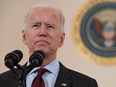
Former US president Donald Trump and current US President Joe Biden will face off in November to win a second term.Credit: Morry Gash, Jim Watson/AFP via Getty

Voters in 15 US states and one territory weighed in at the polls on 5 March, or ‘Super Tuesday’, and the results lock in a rematch between Republican Donald Trump and the incumbent, Democrat Joe Biden, in November’s election for the next US president. The outcome could have massive implications for the environment, public health and international collaborations between scientists — as well as, some fear, US democracy itself.

Trump soundly beat his lone remaining challenger for the Republican nomination, Nikki Haley, a former US ambassador to the United Nations, who dropped out of the race on 6 March. The former president prevailed despite facing 91 criminal charges alleging interference with the 2020 presidential election, economic fraud and mishandling of classified materials. The result of this year’s election could hinge on the outcome of those cases, as well as on potential long-shot presidential challenges from candidates labelling themselves as independents. But for now, Trump has consolidated his control over the Republican Party and will once again run against Biden, whom Democrats have rallied behind.

The two candidates have opposing views on a host of scientific issues. As president, Biden has promoted climate and clean-energy innovation, and bolstered scientific-integrity policies throughout the federal government that are meant to protect evidence-based decision-making. During his presidency from 2017 to 2020, Trump repealed climate policies and promoted fossil fuels, while sidelining public-health officials and other government scientists. Each is expected to lean further into these stances if he wins a second term.

Here, Nature talks to policy analysts and researchers about what’s on the line in November.

Climate action or disruption?

“It’s a trope to say that every election is critical, but this election is particularly stark in the two paths that it presents for the United States,” says Alexander Barron, an environmental scientist at Smith College in Northampton, Massachusetts, who has worked under both Biden and former US president Barack Obama.

As president, Trump pulled the United States out of the Paris climate accord. He would probably do so again if elected while seeking to roll back climate regulations put in place by the Biden administration to curb greenhouse-gas emissions, including from vehicles and power plants. But there might be limits to what Trump would be able to achieve.

Republican presidential candidate and former President Donald Trump reacts to supporters as he arrives on stage at a Get Out the Vote Rally March 2, 2024 in Richmond, Virginia.

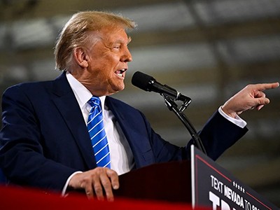
Trump at a campaign rally in Richmond, Virginia, on 2 March.Credit: Win McNamee/Getty

For instance, Biden signed the Inflation Reduction Act (IRA) in 2022, which by some estimates helped to lock in around US$1 trillion in funding for clean-energy programmes over a decade. If Trump wanted to repeal that legislation, it would require an act of Congress, which would be possible only if Republicans maintain control of the US House of Representatives and gain a majority in the Senate, which Democrats now control by a slim margin. And even then, observers say, the politics could be tricky given that large investments are already starting to flow into communities represented by lawmakers on both sides of the political aisle.

Nonetheless, Trump could still disrupt the climate agenda laid out in the IRA, says Greg Dotson, a legal scholar at the University of Oregon in Eugene, who was involved in crafting the legislation as a Democratic staff member in the Senate.

“The first Trump administration was very hostile to climate policies, and they didn’t feel necessarily restrained by the law,” Dotson says, noting that Trump could still block funding and rewrite climate-programme rules if he returned to office. By contrast, climate-policy specialists say that another four years under Biden could lock in nearly a decade of significant progress. This is what will be needed if the country is to have any hope of achieving Biden’s pledge to halve US emissions by 2030 and achieve net zero by mid-century.

“Getting to those targets is going to be a tremendous group effort,” Barron says. “We really need all levels of government and all sectors to continue moving in the right direction.”

The health of the nation

The two candidates also differ notably in their approach to investing in public health. For example, in each of Trump’s four years in office, his administration sought, unsuccessfully, to cut the budget of the US National Institutes of Health (NIH), the country’s premier biomedical-research agency. Biden, on the other hand, kick-started the US$2.5-billion Advanced Research Projects Agency for Health, aimed at tackling high-risk, high-reward biomedical research — which he’d probably continue to support if re-elected.

The Trump administration also attempted to cut funding for the US Centers for Disease Control and Prevention (CDC) — an agency tasked with protecting public health — and undermined its scientists during the COVID-19 pandemic by, for example, countering their claims about the seriousness of the health emergency. By contrast, Biden has proposed budget increases for the CDC and has publicly defended the agency and its scientists. “Trump did a lot to discredit public health and scientific agencies in the United States, and it has been difficult to rebuild the trust,” says Larry Levitt, an executive vice-president at the health-policy research organization KFF, based in San Francisco, California.

First lady Jill Biden, President Joe Biden, Vice President Kamala Harris and Second gentleman Douglas Emhoff on stage during a campaign rally in Virginia.

Biden has pledged to resecure the nationwide right to an abortion, once protected by a Supreme Court ruling in the case Roe v. Wade.Credit: Anna Moneymaker/Getty

That stance will probably continue. At a campaign rally last week, Trump hinted that he would endorse elements of the anti-vaccine movement if re-elected, suggesting that he would deny federal funds to schools with a vaccine mandate.

The United States’ role in global health is also at stake. During his presidency, Trump pulled the United States out of the World Health Organization (WHO) and generally pursued isolationist policies, Levitt says. “Biden has done a lot to undo that, but we will likely see a slip back if Trump were elected again,” he says. Officials in the Biden administration have expressed their commitment to a global pandemic treaty — an agreement being negotiated among countries to help prevent the next global-health emergency. Meanwhile, Republicans have been critical of it, suggesting that it could be a threat to US intellectual-property rights, forcing companies to share vaccine and treatment know-how.

Ever since the 2022 US Supreme Court decision that ended nationwide abortion rights, the issue has become crucial for voters. The two candidates have adopted opposing positions: Trump, who vowed to overturn abortion rights when he took office, now supports a national ban on abortions after 16 weeks of pregnancy, whereas Biden has vowed to once again secure abortion rights, by passing a law to protect them. Both pledges would require congressional action to be fulfilled, so it isn’t clear whether either would be successful. “We’re at one of the most consequential moments for abortion access in modern American history,” says Nourbese Flint, president of All Above All Action Fund, an abortion-justice advocacy group in Washington DC.

Cross-border science

Another area where Biden and Trump differ vastly is in their approach to immigration, as well as the visas that thousands of foreign students and scientists depend on to study and work in the United States. Weeks after Trump’s presidential inauguration, he introduced broad travel bans that stopped citizens from seven majority-Muslim countries, including Iran and Syria, from entering the United States. The move left international students stranded at airports and shocked the scientific community.

When Biden took office in 2021, he quickly overturned the ban. And he has taken other steps to reform immigration for professionals such as scientists: in January 2022, the US Citizenship and Immigration Services clarified guidance for workers in science, technology, engineering and mathematics (STEM) who are seeking visas to come to the United States. This has increased the number of STEM visas being issued, according to the agency.

Should either candidate win the election in November, these stances will probably influence their agendas, experts say. But one area where their policies have more closely aligned — and is unlikely to change — is relations with China.

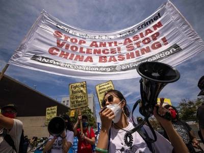
In 2018, under Trump, the US Department of Justice launched the China Initiative, a programme meant to safeguard US laboratories and businesses against espionage. The initiative led to a number of arrests of scientists with Chinese heritage, but when Biden took office, his administration reviewed the initiative and ended it, arguing that the programme had been perceived as using racial profiling to achieve its aims. Biden nonetheless continued with reforms introduced by Trump that required US universities and research organizations that were awarded more than $50 million per year in federal research funding to prove that they have instituted a research-security programme, including tougher scrutiny of foreign travel.

Such policies have made US institutions wary of collaborating with scientists in China, experts say. And in fact, studies have shown that scientific collaborations between the United States and China have continued to decrease under Biden. The number of students coming from China to study in the United States has dropped, too.

At the end of last year, Republican lawmakers in the US House of Representatives wrote that it had been “unwise” of the Biden administration to end the China Initiative, sparking fear among civil-liberties advocates that they would try to reinstate the programme. They hope that a renewed Biden administration would stave off such efforts, but aren’t sure what would happen under a second Trump term.

“Relations with China won’t improve in the foreseeable future, but they could get worse,” says Jenny Lee, a higher-education researcher and vice-president for international affairs at the University of Arizona in Tucson.

The elections in November will undoubtedly affect government policies on many scientific issues. But for Barron, similar to many others, science is just one of many concerns that he has about a potential second term for Trump, who has questioned the legitimacy of the 2020 election, promoted misinformation on a number of fronts, and signalled that he will institute new rules that critics argue will make it easier to fire career government employees who oppose his politics. “I would put myself in the camp that is most worried about democracy,” Barron says.

[ad_2]

Source Article Link

Categories
Featured

Grado Reference Series The Hemp headphones review: sonically spot on

[ad_1]

Grado Hemp: Two-minute review

The Reference Series Hemp headphones started out as a limited edition – but thanks to popular opinion, Grado has decided to make them a permanent part of its catalog. How likely are the Grado Hemp to feature in our best wired headphones buying guide? Very, with just a few caveats. 

In many ways – certainly aesthetic – it’s Grado business as usual. Which isn’t all good news, exactly, because it means these headphones are nothing special where perceived value is concerned, are far from luxurious as objects, and become less than comfortable more quickly than, say, the Sennheiser HD 660S2 they’re likely to face off against on most people’s shortlists.

Happily, it’s also business as usual where sound quality is concerned. The combination of the open-backed configuration, along with the acoustic talents of the maple-and-hemp construction of the driver housing, means these headphones sound spacious, detailed and thoroughly engaging. So much so, in fact, that you’ll almost certainly find they’re becoming just slightly uncomfortable before you’re really ready to stop listening to them.  

Grado Hemp headphones on a white table

Striking wooden ear cups in an otherwise so-very-Grado build (Image credit: Future)

Grado Hemp review: Price & release date

  • Release date: February 1, 2024
  • Price: $479 / £479 / AU$799

[ad_2]

Source Article Link

Categories
Life Style

The world must rethink plans for ageing oil and gas platforms

[ad_1]

One of world’s largest oil platforms, the North Sea’s Gullfaks C, sits on immense foundations, constructed from 246,000 cubic metres of reinforced concrete, penetrating 22 metres into the sea bed and smothering about 16,000 square metres of sea floor. The platform’s installation in 1989 was a feat of engineering. Now, Gullfaks C has exceeded its expected 30-year lifespan and is due to be decommissioned in 2036. How can this gargantuan structure, and others like it, be taken out of action in a safe, cost-effective and environmentally beneficial way? Solutions are urgently needed.

Many of the world’s 12,000 offshore oil and gas platforms are nearing the end of their lives (see ‘Decommissioning looms’). The average age of the more than 1,500 platforms and installations in the North Sea is 25 years. In the Gulf of Mexico, around 1,500 platforms are more than 30 years old. In the Asia–Pacific region, more than 2,500 platforms will need to be decommissioned in the next 10 years. And the problem won’t go away. Even when the world transitions to greener energy, offshore wind turbines and wave-energy devices will, one day, also need to be taken out of service.

DECOMMISSIONING LOOMS: chart showing the number of offshore oil, gas and wind structures installed vs decommissioned since 1960.

Source: S. Gourvenec et al. Renew. Sustain. Energy Rev. 154, 111794 (2022).

There are several ways to handle platforms that have reached the end of their lives. For example, they can be completely or partly removed from the ocean. They can be toppled and left on the sea floor. They can be moved elsewhere, or abandoned in the deep sea. But there’s little empirical evidence about the environmental and societal costs and benefits of each course of action — how it will alter marine ecosystems, say, or the risk of pollution associated with moving or abandoning oil-containing structures.

So far, politics, rather than science, has been the driving force for decisions about how to decommission these structures. It was public opposition to the disposal of a floating oil-storage platform called Brent Spar in the North Sea that led to strict legislation being imposed in the northeast Atlantic in the 1990s. Now, there is a legal requirement to completely remove decommissioned energy infrastructure from the ocean in this region. By contrast, in the Gulf of Mexico, the idea of converting defunct rigs into artificial reefs holds sway despite a lack of evidence for environmental benefits, because the reefs are popular sites for recreational fishing.

A review of decommissioning strategies is urgently needed to ensure that governments make scientifically motivated decisions about the fate of oil rigs in their regions, rather than sleepwalking into default strategies that could harm the environment. Here, we outline a framework through which local governments can rigorously assess the best way to decommission offshore rigs. We argue that the legislation for the northeast Atlantic region should be rewritten to allow more decommissioning options. And we propose that similar assessments should inform the decommissioning of current and future offshore wind infrastructure.

Challenges of removing rigs

For the countries around the northeast Atlantic, leaving disused oil platforms in place is an emotive issue as well as a legal one. Environmental campaigners, much of the public and some scientists consider anything other than the complete removal of these structures to be littering by energy companies1. But whether rig removal is the best approach — environmentally or societally — to decommissioning is questionable.

There has been little research into the environmental impacts of removing platforms, largely owing to lack of foresight2. But oil and gas rigs, both during and after their operation, can provide habitats for marine life such as sponges, corals, fish, seals and whales3. Organisms such as mussels that attach to structures can provide food for fish — and they might be lost if rigs are removed4. Structures left in place are a navigational hazard for vessels, making them de facto marine protected areas — regions in which human activities are restricted5. Another concern is that harmful heavy metals in sea-floor sediments around platforms might become resuspended in the ocean when foundations are removed6.

Removing rigs is also a formidable logistical challenge, because of their size. The topside of a platform, which is home to the facilities for oil or gas production, can weigh more than 40,000 tonnes. And the underwater substructure — the platform’s foundation and the surrounding fuel-storage facilities — can be even heavier. In the North Sea, substructures are typically made of concrete to withstand the harsh environmental conditions, and can displace more than one million tonnes of water. In regions such as the Gulf of Mexico, where conditions are less extreme, substructures can be lighter, built from steel tubes. But they can still weigh more than 45,000 tonnes, and are anchored to the sea floor using two-metre-wide concrete pilings.

Huge forces are required to break these massive structures free from the ocean floor. Some specialists even suggest that the removal of the heaviest platforms is currently technically impossible.

And the costs are astronomical. The cost to decommission and remove all oil and gas infrastructure from UK territorial waters alone is estimated at £40 billion (US$51 billion). A conservative estimate suggests that the global decommissioning cost for all existing oil and gas infrastructure could be several trillion dollars.

Mixed evidence for reefing

In the United States, attitudes to decommissioning are different. A common approach is to remove the topside, then abandon part or all of the substructure in such a way that it doesn’t pose a hazard to marine vessels. The abandoned structures can be used for water sports such as diving and recreational fishing.

This approach, known as ‘rigs-to-reefs’, was first pioneered in the Gulf of Mexico in the 1980s. Since its launch, the programme has repurposed around 600 rigs (10% of all the platforms built in the Gulf), and has been adopted in Brunei, Malaysia and Thailand.

Converting offshore platforms into artificial reefs is reported to produce almost seven times less air-polluting emissions than complete rig removal7, and to cost 50% less. Because the structures provide habitats for marine life5, proponents argue that rigs increase the biomass in the ocean8. In the Gulf of California, for instance, increases in the number of fish, such as endangered cowcod (Sebastes levis) and other commercially valuable rockfish, have been reported in the waters around oil platforms6.

But there is limited evidence that these underwater structures actually increase biomass9. Opponents argue that the platforms simply attract fish from elsewhere10 and leave harmful chemicals in the ocean11. And because the hard surface of rigs is different from the soft sediments of the sea floor, such structures attract species that would not normally live in the area, which can destabilize marine ecosystems12.

Evidence from experts

With little consensus about whether complete removal, reefing or another strategy is the best option for decommissioning these structures, policies cannot evolve. More empirical evidence about the environmental and societal costs and benefits of the various options is needed.

To begin to address this gap, we gathered the opinions of 39 academic and government specialists in the field across 4 continents13,14. We asked how 12 decommissioning options, ranging from the complete removal of single structures to the abandonment of all structures, might impact marine life and contribute to international high-level environmental targets. To supplement the scant scientific evidence available, our panel of specialists used local knowledge, professional expertise and industry data.

A starfish, blacksmith fish and other marine life covers the underwater structure on the Eureka Oil Rig

The substructures of oil rigs can provide habitats for a wealth of marine life.Credit: Brent Durand/Getty

The panel assessed the pressures that structures exert on their environment — factors such as chemical contamination and change in food availability for marine life — and how those pressures affect marine ecosystems, for instance by altering biodiversity, animal behaviour or pollution levels. Nearly all pressures exerted by leaving rigs in place were considered bad for the environment. But some rigs produced effects that were considered beneficial for humans — creating habitats for commercially valuable species, for instance. Nonetheless, most of the panel preferred, on balance, to see infrastructure that has come to the end of its life be removed from the oceans.

But the panel also found that abandoning or reefing structures was the best way to help governments meet 37 global environmental targets listed in 3 international treaties. This might seem counter-intuitive, but many of the environmental targets are written from a ‘what does the environment do for humans’ perspective, rather than being focused on the environment alone.

Importantly, the panel noted that not all ecosystems respond in the same way to the presence of rig infrastructure. The changes to marine life caused by leaving rigs intact in the North Sea will differ from those brought about by abandoning rigs off the coast of Thailand. Whether these changes are beneficial enough to warrant alternatives to removal depends on the priorities of stakeholders in the region — the desire to protect cowcod is a strong priority in the United States, for instance, whereas in the North Sea, a more important consideration is ensuring access to fishing grounds. Therefore, rig decommissioning should be undertaken on a local, case-by-case basis, rather than using a one-size-fits-all approach.

Legal hurdles in the northeast Atlantic

If governments are to consider a range of decommissioning options in the northeast Atlantic, policy change is needed.

Current legislation is multi-layered. At the global level, the United Nations Convention on the Law of the Sea (UNCLOS; 1982) states that no unused structures can present navigational hazards or cause damage to flora and fauna. Thus, reefing is allowed.

But the northeast Atlantic is subject to stricter rules, under the OSPAR Convention. Named after its original conventions in Oslo and Paris, OSPAR is a legally binding agreement between 15 governments and the European Union on how best to protect marine life in the region (see go.nature.com/3stx7gj) that was signed in the face of public opposition to sinking Brent Spar. The convention includes Decision 98/3, which stipulates complete removal of oil and gas infrastructure as the default legal position, returning the sea floor to its original state. This legislation is designed to stop the offshore energy industry from dumping installations on mass.

Under OSPAR Decision 98/3, leaving rigs as reefs is prohibited. Exceptions to complete removal (derogations) are occasionally allowed, but only if there are exceptional concerns related to safety, environmental or societal harms, cost or technical feasibility. Of the 170 structures that have been decommissioned in the northeast Atlantic so far, just 10 have been granted derogations. In those cases, the concrete foundations of the platforms have been left in place, but the top part of the substructures removed.

Enable local decision-making

The flexibility of UNCLOS is a more pragmatic approach to decommissioning than the stringent removal policy stipulated by OSPAR.

We propose that although the OSPAR Decision 98/3 baseline position should remain the same — complete removal as the default — the derogation process should change to allow alternative options such as reefing, if a net benefit to the environment and society can be achieved. Whereas currently there must be an outstanding reason to approve a derogation under OSPAR, the new process would allow smaller benefits and harms to be weighed up.

The burden should be placed on industry officials to demonstrate clearly why an alternative to complete removal should be considered not as littering, but as contributing to the conservation of marine ecosystems on the basis of the best available scientific evidence. The same framework that we used to study global-scale evidence in our specialist elicitation can be used to gather and assess local evidence for the pros and cons of each decommissioning option. Expert panels should comprise not only scientists, but also members with legal, environmental, societal, cultural and economic perspectives. Regions outside the northeast Atlantic should follow the same rigorous assessment process, regardless of whether they are already legally allowed to consider alternative options.

For successful change, governments and legislators must consider two key factors.

Get buy-in from stakeholders

OSPAR’s 16 signatories are responsible for changing its legislation but it will be essential that the more flexible approach gets approval from OSPAR’s 22 intergovernmental and 39 non-governmental observer organizations. These observers, which include Greenpeace, actively contribute to OSPAR’s work and policy development, and help to implement its convention. Public opinion in turn will be shaped by non-governmental organizations15 — Greenpeace was instrumental in raising public awareness about the plan to sink Brent Spar in the North Sea, for instance.

Transparency about the decision-making process will be key to building confidence among sceptical observers. Oil and gas companies must maintain an open dialogue with relevant government bodies about plans for decommissioning. In turn, governments must clarify what standards they will require to consider an alternative to removal. This includes specifying what scientific evidence should be collated, and by whom. All evidence about the pros and cons of each decommissioning option should be made readily available to all.

Oil and gas companies should identify and involve a wide cross-section of stakeholders in decision-making from the earliest stages of planning. This includes regulators, statutory consultees, trade unions, non-governmental organizations, business groups, local councils and community groups and academics, to ensure that diverse views are considered.

Conflict between stakeholders, as occurred with Brent Spar, should be anticipated. But this can be overcome through frameworks similar to those between trade unions and employers that help to establish dialogue between the parties15.

The same principle of transparency should also be applied to other regions. If rigorous local assessment reveals reefing not to be a good option for some rigs in the Gulf of Mexico, for instance, it will be important to get stakeholder buy-in for a change from the status quo.

Future-proof designs

OSPAR and UNCLOS legislation applies not only to oil and gas platforms but also to renewable-energy infrastructure. To avoid a repeat of the challenges that are currently being faced by the oil and gas industry, decommissioning strategies for renewables must be established before they are built, not as an afterthought. Structures must be designed to be easily removed in an inexpensive way. Offshore renewable-energy infrastructure should put fewer pressures on the environment and society — for instance by being designed so that it can be recycled, reused or repurposed.

If developers fail to design infrastructure that can be removed in an environmentally sound and cost-effective way, governments should require companies to ensure that their structures provide added environmental and societal benefits. This could be achieved retrospectively for existing infrastructure, taking inspiration from biodiversity-boosting panels that can be fitted to the side of concrete coastal defences to create marine habitats (see go.nature.com/3v99bsb).

Governments should also require the energy industry to invest in research and development of greener designs. On land, constraints are now being placed on building developments to protect biodiversity — bricks that provide habitats for bees must be part of new buildings in Brighton, UK, for instance (see go.nature.com/3pcnfua). Structures in the sea should not be treated differently.

If it is designed properly, the marine infrastructure that is needed as the world moves towards renewable energy could benefit the environment — both during and after its operational life. Without this investment, the world could find itself facing a decommissioning crisis once again, as the infrastructure for renewables ages.

[ad_2]

Source Article Link

Categories
Featured

Brane X review: a portable smart speaker with incredible bass

[ad_1]

Brane Audio Brane X: Two-minute review

Brane Audio’s Brane X has managed to achieve the unthinkable in the mostly mundane realm of the best wireless speakers, which – to be clear – is full of models that don’t leave much of an impression. Some are good, some are okay, and many are bad. But the Brane X makes an impression. 

The main way the Brane X impresses is by delivering bass output extending into the sub-bass range. That’s unheard of for a portable speaker. Still, the Brane X isn’t an ordinary portable speaker, but one with proprietary Repel-Attract-Driver (R.A.D.) technology that uses a magnet array to cancel out air pressure within the speaker’s enclosure. This allows big bass to be generated from a small woofer in a highly compact box, and it needs to be heard to be believed.

[ad_2]

Source Article Link

Categories
Life Style

Will these reprogrammed elephant cells ever make a mammoth?

[ad_1]

An artist's impression of three woolly mammoths in a snowy landscape.

Woolly mammoths’ closest living relatives are Asian elephants, which could be genetically engineered to have mammoth-like traits.Credit: Mark Garlick/Science Photo Library via Alamy

Scientists have finally managed to put elephant skin cells into an embryonic state.

The breakthrough — announced today by the de-extinction company Colossal Biosciences in Dallas, Texas — is an early technical success in Colossal’s high-profile effort to engineer elephants with woolly mammoth traits.

Eighteen years ago, researchers showed that mouse skin cells could be reprogrammed to act like embryonic cells1. These induced pluripotent stem (iPS) cells can differentiate into any of an animal’s cell types. They are key to Colossal’s plans to create herds of Asian elephants (Elephus maximus) — the closest living relative of extinct woolly mammoths (Mammuthus primigenius) — that have been genetically edited to have shaggy hair, extra fat and other mammoth traits.

“I think we’re certainly in the running for the world-record hardest iPS-cell establishment,” says Colossal co-founder George Church, a geneticist at Harvard Medical School in Boston, Massachusetts, and a co-author of a preprint describing the work, which will soon appear on the server bioRxiv.

But the difficulty of establishing elephant iPS cells — in theory, one of the most straightforward steps in Colossal’s scheme — underscores the huge technical hurdles the team faces.

Endangered species

In 2011, Jeanne Loring, a stem-cell biologist at the Scripps Research Institute in La Jolla, California, and her colleagues created iPS cells from a northern white rhinoceros (Ceratotherium simum cottoni) and a monkey called a drill (Mandrillus leucophaeus), the first such cells from endangered animals2. Embryonic-like stem cells have since been made from a menagerie of threatened species, including snow leopards (Panthera uncia)3, Sumatran orangutans (Pongo abelii)4 and Japanese ptarmigans (Lagopus muta japonica)5. However, numerous teams have failed in their attempts to establish elephant iPS cells. “The elephant has been challenging,” says Loring.

A team led by Eriona Hysolli, Colossal’s head of biological sciences, initially ran into the same problems trying to reprogram cells from an Asian elephant calf by following the recipe used to make most other iPS cell lines: instructing the cells to overproduce four key reprogramming factors identified by Shinya Yamanaka, a stem-cell scientist at Kyoto University in Japan, in 20061.

When this failed, Hysolli and her colleagues treated elephant cells with a chemical cocktail that others had used to reprogram human and mice cells. In most cases, the treatment caused the elephant cells to die, stop dividing or simply do nothing. But in some experiments, the cells took on a rounded shape similar to that of stem cells. Hysolli’s team added the four ‘Yamanaka’ factors to these cells, then took another step that turned out to be key to success: dialling down the expression of an anti-cancer gene called TP53.

The researchers created four iPS-cell lines from an elephant. The cells looked and behaved like iPS cells from other organisms: they could form cells that make up the three ‘germ layers’ that comprise all a vertebrate’s tissues.

“We’ve been really waiting for these things desperately,” says Church.

Technological leaps

Colossal’s plan to create its first gene-edited Asian elephants involves cloning technology that does not require iPS cells. But Church says the new cell lines will be useful for identifying and studying the genetic changes needed to imbue Asian elephants with mammoth traits. “We’d like to pre-test them before we put them in baby elephants,” Church says. Elephant iPS cells could be edited and then transformed into relevant tissue, such as hair or blood.

But scaling up the process would require numerous other leaps in reproductive biology. One path involves transforming gene-edited iPS cells into sperm and egg cells to make embryos, which has been accomplished in mice6. It might also be possible to convert iPS cells directly into viable ‘synthetic’ embryos.

To avoid the need for herds of Asian elephant surrogates to carry such embryos to term, Church imagines that artificial wombs, derived in part from iPS cells, would be used. “We do not want to interfere with the natural reproduction of endangered species, so we’re trying to scale up in vitro gestation,” he says

Time and effort

Loring, who last year co-organized a conference on iPS cells from endangered animals, says adding elephants to the list is important, but not game-changing. “It will be useful for others who are having challenges reprogramming the species they’re interested in,” she says.

Sebastian Diecke, a stem-cell biologist at the Max Delbrück Center for Molecular Medicine in the Helmholtz Association in Berlin, would like to see more evidence that iPS cell lines grow stably and can be transformed into different kinds of tissues, for instance, by making brain organoids with them. “There are still steps before we can call them proper iPS cells,” he says.

Vincent Lynch, an evolutionary geneticist at the University at Buffalo in New York, has been trying — and failing — to make elephant iPS cells for years. He plans to attempt the method Hysolli and her colleagues developed, as part of his lab’s ongoing efforts to understand why elephants seem to develop cancer only rarely.

The myriad technologies needed to grow an iPS cell into a mammoth-like elephant might not be even close to ready yet. But given enough time and money, it should be possible, Lynch says. “I just don’t know the time frame and whether it’s worth the resources.”

[ad_2]

Source Article Link

Categories
Featured

What time does the Oscars 2024 start?

[ad_1]

Lights, camera, confusion? A change to the 2024 Oscars start time has threatened to upstage the stars themselves at the 96th Academy Awards this weekend. In a move intended to boost viewing figures, the Academy of Motion Picture Arts and Sciences has broken with tradition and shifted the ceremony to 7pm ET, though Sunday also happens to be the day the clocks change in the US. 

It’s good news for most viewers, especially those based east of the west coast, because it means the jewel in the crown, the best picture award, will be presented significantly earlier than usual. Read on so you don’t miss the battle between Oppenheimer, American Fiction, The Holdovers and The Zone of Interest.

When are the Oscars?

[ad_2]

Source Article Link

Categories
Life Style

A rapidly time-varying equatorial jet in Jupiter’s deep interior

[ad_1]

In Fig. 1, we superimpose a steady, axisymmetric, zonal flow profile on a background map of the magnetic field2 derived from Juno magnetic field observations11 from the spacecraft’s first 33 orbits. The flow is dominated by an equatorial jet, which induces intense secular variation in the vicinity of the Great Blue Spot (the region of concentrated field at the equator) as the magnetic field associated with this spot is swept eastwards. Owing to its dominant role in generating the secular variation1,2,3,12, a recent set of orbits by the Juno spacecraft13 was targeted at this region.

Fig. 1: The steady velocity field and the background radial component of the magnetic field at 0.9 RJ .
figure 1

The projection is Hammer equal-area with the central meridian at 180° in System III coordinates (highlighted in grey); the central meridian is the zero line for the steady flow. The colour scale for the background magnetic field model is linear between the indicated limits. The flow velocity is scaled with latitude to account for the poleward convergence of meridians; the peak velocity (corresponding to the equatorial jet) is 0.86 cm s−1.

To begin, we produce a new model including the magnetic field observations from these targeted passes (and other subsequent orbits over other regions of the planet). The model is produced using the same method as the model in Fig. 1 (Methods and ref. 2). One pass, PJ02 (in which PJ stands for perijove), did not acquire any data, so the number of data-yielding orbits is 41 compared with 32 orbits for the earlier model; note we refer to these models in terms of the last orbit used, that is, the 33-orbit model (Fig. 1) and the 42-orbit model. The resulting 42-orbit model has a global misfit of 492 nT compared with 411 nT for the 33-orbit model (for comparison, the root-mean-square (r.m.s.) field strength of the observations is 282,000 nT); within a box around the spot (Fig. 2) the misfit is 934 nT compared with 675 nT (where the r.m.s. field strength is 393,000 nT) and the maximum speed of the equatorial jet is 0.64 cm s−1 compared with 0.86 cm s−1. Thus, the fits we obtain to the 42-orbit dataset are poorer than those to the earlier 33-orbit dataset, especially near the spot, indicating that a steady flow performs worse as the time interval spanned by the passes increases. We may have expected, instead, that with the addition of these later passes that the misfit would decrease because these passes are at higher altitude over the spot and hence sample weaker field. Except for the southern hemisphere south of 30 °S, where the flow resolution is poor2, the flow profiles are broadly similar; however, the equatorial jet speed is reduced by 26% in the 42-orbit solution, suggesting that the flow may be changing with time. The pattern of residuals in Fig. 2a lends additional support to this possibility: we can identify pairs of passes that are spatially adjacent but separated in time that have oppositely signed residuals over the spot, notably PJ19 and PJ36, and PJ24 and PJ38. Oppositely signed residuals will result for adjacent passes if the actual flow speed at the time of the passes is greater than the steady flow solution for one pass and smaller for the other.

Fig. 2: Residuals of the radial component of the magnetic field data along track.
figure 2

The residuals (the difference between the observation and the model prediction), calculated every 15 s, are plotted along the track, with positive residuals plotted west of the track (in red) and negative residuals east of the track (in blue) as the spacecraft passes through periapsis from north to south. The radial component of the magnetic field model is shown in the background. The projection is cylindrical with a grid spacing of 15°; the equator is highlighted in grey. The residuals are calculated within the box shown in black. The colour scale is linear between the indicated limits and the bar below the colour scale depicts the residual scale. a, The residuals from the 42-orbit steady flow model. b, The residuals from the 42-orbit steady flow model after applying the pass-by-pass velocity scale factors. c, The residuals from the 42-orbit steady flow model after applying the sinusoidal flow time-variation model.

To examine the possibility that the flow speed is varying, we allow the flow to vary in amplitude on a pass-by-pass basis. We do this by applying a velocity scale factor to the flow for each pass (Methods). The velocity scale factor does not change the flow profile, instead it simply scales its amplitude. By doing so, we find the adjusted flow speed that gives the best fit for a particular pass, but for a different pass that flow speed will probably be different. These adjusted flow speeds represent the average flow speed from the baseline epoch of 2016.5 for each particular pass. In Fig. 2b we show the residuals after applying velocity scale factors to each pass. The residuals are reduced, especially for passes to the west of the spot. The misfit within the box is 721 nT, a variance reduction of 40% from the steady flow solution. This variance reduction can be considered as the maximum that can be achieved simply by varying the flow speed. However, this variation is only physically reasonable if we can find a time-varying flow consistent with the pass-by-pass velocity scale factors, in other words a time-varying flow that yields the corresponding average flow speed for each pass. It is possible, instead, that the different velocity scale factors (or average flow speeds) are mutually inconsistent.

We examine whether such a flow exists by fitting the pass-by-pass velocity scale factors with a simple sinusoidally varying flow model with a single period and no damping (Methods). We omit PJ01 from this analysis as that orbit passes over the spot less than 2 months after the baseline epoch and thus is insensitive to variations in the flow (the flow would advect the spot by less than 0.05° during those 2 months). The best-fit solution is shown in Figs. 2c and 3: it has a period of 3.8 years and results in a variance reduction within the box of 24.8%. As expected, the variance reduction on a pass-by-pass basis varies substantially (Fig. 3b), as those passes with velocity scale factors that differ substantially from unity will have their fit enhanced more than a pass with a factor close to unity. Note that Fig. 3 shows the residuals to the radial component of the field, rather to the three components of the magnetic field, as the radial component is more readily interpreted in terms of changes in the flow speed. In a few cases, though, other components of the field show a much larger reduction in misfit than the radial component, most particularly Bϕ (the east component of the magnetic field) for PJ24. In other words, there is not necessarily a one-to-one correspondence between the residuals in Fig. 2 and the variance reductions in Fig. 3. Comparing Fig. 2a with 2c, we can see that the residuals of the pairs of passes discussed earlier (PJ19 and 36, and 24 and 38) are much reduced. For most passes, the red bars in Fig. 3b (the normalized misfits to the sinusoidal model) are below the grey line corresponding to 1 (the normalized misfit of the 42-orbit steady flow model), but two passes (PJ26 and PJ37) stand well-above the grey line indicating that they are fit worse by the sinusoidal model than by the 42-orbit steady flow model. These two passes are the most easterly passes within the box. PJ37 requires a flow speed almost 15% more rapid than that of PJ36 and PJ38, which though temporally adjacent to PJ37 are not spatially adjacent to PJ37, indicating that additional spatial complexity in the flow may be required. PJ26 is, instead, fit by a slower flow than the sinusoidal model arguing instead for additional temporal complexity. Additional complexity could take the form of more than one wave being present or wave damping. In case our results are skewed by these two passes, we repeat the sinusoidal fit omitting them, as shown by the light red curve in Fig. 3a. The fit to most of the remaining passes, in particular PJ24 and the targeted passes (PJ36, PJ38, PJ39, PJ41 and PJ42) is improved. The period of the sinusoidal fit is changed by only a small amount from 3.8 to 4.1 years.

Fig. 3: Velocity scale factors, time-averaged sinusoid fit and misfits.
figure 3

a, The cyan symbols represent the velocity scale factors for each pass. The error bars represent one standard deviation (Methods). The red curve shows the sinusoidal fit using all the passes and the light red curve the fit omitting PJ26 and PJ37 (for details of the fit, see Methods, equation (12). b, The misfit to each pass, normalized by the misfit to the 42-orbit steady flow model. The cyan bars represent the normalized misfit after applying velocity scale factors on a pass-by-pass basis; the red bars represent the normalized misfit after applying the sinusoidal model. In both panels, we depict the 42-orbit steady flow model by a horizontal line. a, The line corresponds to the unadjusted velocity of the 42-orbit steady flow model, in other words a velocity scale factor of unity for all passes. b, The horizontal line shows a misfit of 1, as the misfits have been normalized to the 42-orbit steady flow model.

Source data

The period of roughly 4 years suggests that this is a torsional oscillation or Alfvén wave rather than, for example, a MAC (magnetic-Archimedean-Coriolis) wave14, which would have a much longer period. Torsional oscillations have also been proposed as the origin of cloud level variability in Jupiter on subdecadal timescales15: the zonal shear associated with a torsional oscillation may modulate the heat flux from the deep interior, which may in turn result in variability of observed infrared emissions at cloud level. The wave speed of torsional oscillations is determined by the r.m.s. value of the component of the magnetic field, \({\bar{B}}_{{\rm{s}}}\), perpendicular to the rotation axis10 (where the average is taken over longitude and the latitude band of interest). For an equatorial belt of ±10° about the equator (the latitudinal extent of the deep equatorial jet), we find \({\bar{B}}_{{\rm{s}}}=0.6\) mT at 0.9 RJ. This corresponds to an Alfvén wave speed of 10−2 ms−1.

The period of the oscillation depends, of course, on its wavenumber k, for which we have no direct observation. If the cloud level variability is due to torsional oscillations, then the wavenumber can be estimated from the length scale of those variations, yielding dimensionless wavenumbers kRJ/2π in the range 10 to 15 (ref. 15). Here, however, we are examining a single equatorial fluctuation rather than a set of torsional oscillations spanning a wide range of latitudes. For the equatorial jet, a dimensionless wavenumber of 10 could be considered (although this would be based on the azimuthal extent of the jet rather than its wavenumber in the s direction) yielding a period of roughly 15 years: that is, four times longer than that found here.

However, our estimate of \({\bar{B}}_{{\rm{s}}}\) may be too small: the field is most probably stronger at depths below 0.9 RJ, but the field below that depth cannot be reliably estimated from the externally observed potential field owing to the rapid increase of electrical conductivity with depth16; and second, intense, small scale magnetic fields (which will be geometrically attenuated in the observations at satellite altitude) may serve to increase \({\bar{B}}_{{\rm{s}}}\) further.

A period of 4 years corresponds to a field strength \({\bar{B}}_{{\rm{s}}}\approx 3\) mT, similar to the field strength associated with the spot itself, so the wave may instead be a localized Alfvén wave propagating along the field lines associated with the spot (which are largely in the s direction), rather than an axisymmetric torsional oscillation, in which case a superimposed longer period torsional oscillation may then also be excited.

[ad_2]

Source Article Link

Categories
Life Style

Integrated optical frequency division for microwave and mmWave generation

[ad_1]

Microwave and mmWave with high spectral purity are critical for a wide range of applications1,2,3, including metrology, navigation and spectroscopy. Owing to the superior fractional frequency stability of reference-cavity stabilized lasers when compared to electrical oscillators14, the most stable microwave sources are now achieved in optical systems by using optical frequency division4,5,6,7 (OFD). Essential to the division process is an optical frequency comb4, which coherently transfers the fractional stability of stable references at optical frequencies to the comb repetition rate at radio frequency. In the frequency division, the phase noise of the output signal is reduced by the square of the division ratio relative to that of the input signal. A phase noise reduction factor as large as 86 dB has been reported4. However, so far, the most stable microwaves derived from OFD rely on bulk or fibre-based optical references4,5,6,7, limiting the progress of applications that demand exceedingly low microwave phase noise.

Integrated photonic microwave oscillators have been studied intensively for their potential of miniaturization and mass-volume fabrication. A variety of photonic approaches have been shown to generate stable microwave and/or mmWave signals, such as direct heterodyne detection of a pair of lasers15, microcavity-based stimulated Brillouin lasers16,17 and soliton microresonator-based frequency combs18,19,20,21,22,23 (microcombs). For solid-state photonic oscillators, the fractional stability is ultimately limited by thermorefractive noise (TRN), which decreases with the increase of cavity mode volume24. Large-mode-volume integrated cavities with metre-scale length and a greater than 100 million quality (Q)-factor have been shown recently8,25 to reduce laser linewidth to Hz-level while maintaining chip footprint at centimetre-scale9,26,27. However, increasing cavity mode volume reduces the effective intracavity nonlinearity strength and increases the turn-on power for Brillouin and Kerr parametric oscillation. This trade-off poses a difficult challenge for an integrated cavity to simultaneously achieve high stability and nonlinear oscillation for microwave generation. For oscillators integrated with photonic circuits, the best phase noise reported at 10 kHz offset frequency is demonstrated in the SiN photonic platform, reaching −109 dBc Hz−1 when the carrier frequency is scaled to 10 GHz (refs. 21,26). This is many orders of magnitude higher than that of the bulk OFD oscillators. An integrated photonic version of OFD can fundamentally resolve this trade-off, as it allows the use of two distinct integrated resonators in OFD for different purposes: a large-mode-volume resonator to provide exceptional fractional stability and a microresonator for the generation of soliton microcombs. Together, they can provide major improvements to the stability of integrated oscillators.

Here, we notably advance the state of the art in photonic microwave and mmWave oscillators by demonstrating integrated chip-scale OFD. Our demonstration is based on complementary metal-oxide-semiconductor-compatible SiN integrated photonic platform28 and reaches record-low phase noise for integrated photonic-based mmWave oscillator systems. The oscillator derives its stability from a pair of commercial semiconductor lasers that are frequency stabilized to a planar-waveguide-based reference cavity9 (Fig. 1). The frequency difference of the two reference lasers is then divided down to mmWave with a two-point locking method29 using an integrated soliton microcomb10,11,12. Whereas stabilizing soliton microcombs to long-fibre-based optical references has been shown very recently30,31, its combination with integrated optical references has not been reported. The small dimension of microcavities allows soliton repetition rates to reach mmWave and THz frequencies12,30,32, which have emerging applications in 5G/6G wireless communications33, radio astronomy34 and radar2. Low-noise, high-power mmWaves are generated by photomixing the OFD soliton microcombs on a high-speed flip-chip bonded charge-compensated modified uni-travelling carrier photodiode (CC-MUTC PD)12,35. To address the challenge of phase noise characterization for high-frequency signals, a new mmWave to microwave frequency division (mmFD) method is developed to measure mmWave phase noise electrically while outputting a low-noise auxiliary microwave signal. The generated 100 GHz signal reaches a phase noise of −114 dBc Hz−1 at 10 kHz offset frequency (equivalent to −134 dBc Hz−1 for 10 GHz carrier frequency), which is more than two orders of magnitude better than previous SiN-based photonic microwave and mmWave oscillators21,26. The ultra-low phase noise can be maintained while pushing the mmWave output power to 9 dBm (8 mW), which is only 1 dB below the record for photonic oscillators at 100 GHz (ref. 36). Pictures of chip-based reference cavity, soliton-generating microresonators and CC-MUTC PD are shown in Fig. 1b.

Fig. 1: Conceptual illustration of integrated OFD.
figure 1

a, Simplified schematic. A pair of lasers that are stabilized to an integrated coil reference cavity serve as the optical references and provide phase stability for the mmWave and microwave oscillator. The relative frequency difference of the two reference lasers is then divided down to the repetition rate of a soliton microcomb by feedback control of the frequency of the laser that pumps the soliton. A high-power, low-noise mmWave is generated by photodetecting the OFD soliton microcomb on a CC-MUTC PD. The mmWave can be further divided down to microwave through a mmWave to microwave frequency division with a division ratio of M. PLL, phase lock loop. b, Photograph of critical elements in the integrated OFD. From left to right are: a SiN 4 m long coil waveguide cavity as an optical reference, a SiN chip with tens of waveguide-coupled ring microresonators to generate soliton microcombs, a flip-chip bonded CC-MUTC PD for mmWave generation and a US 1-cent coin for size comparison. Microscopic pictures of a SiN ring resonator and a CC-MUTC PD are shown on the right. Scale bars, 100 μm (top and bottom left), 50 μm (bottom right).

The integrated optical reference in our demonstration is a thin-film SiN 4-metre-long coil cavity9. The cavity has a cross-section of 6 μm width × 80 nm height, a free-spectral-range (FSR) of roughly 50 MHz, an intrinsic quality factor of 41 × 106 (41 × 106) and a loaded quality factor of 34 × 106 (31 × 106) at 1,550 nm (1,600 nm). The coil cavity provides exceptional stability for reference lasers because of its large-mode volume and high-quality factor9. Here, two widely tuneable lasers (NewFocus Velocity TLB-6700, referred to as laser A and B) are frequency stabilized to the coil cavity through Pound–Drever–Hall locking technique with a servo bandwidth of 90 kHz. Their wavelengths can be tuned between 1,550 nm (fA = 193.4 THz) and 1,600 nm (fB = 187.4 THz), providing up to 6 THz frequency separation for OFD. The setup schematic is shown in Fig. 2.

Fig. 2: Experimental setup.
figure 2

A pair of reference lasers is created by stabilizing frequencies of lasers A and B to a SiN coil waveguide reference cavity, which is temperature controlled by a thermoelectric cooler (TEC). Soliton microcomb is generated in an integrated SiN microresonator. The pump laser is the first modulation sideband of a modulated continuous wave laser, and the sideband frequency can be rapidly tuned by a VCO. To implement two-point locking for OFD, the 0th comb line (pump laser) is photomixed with reference laser A, while the –Nth comb line is photomixed with reference laser B. The two photocurrents are then subtracted on an electrical mixer to yield the phase difference between the reference lasers and N times the soliton repetition rate, which is then used to servo control the soliton repetition rate by controlling the frequency of the pump laser. The phase noise of the reference lasers and the soliton repetition rate can be measured in the optical domain by using dual-tone delayed self-heterodyne interferometry. Low-noise, high-power mmWaves are generated by detecting soliton microcombs on a CC-MUTC PD. To characterize the mmWave phase noise, a mmWave to  microwave frequency division is implemented to stabilize a 20 GHz VCO to the 100 GHz mmWave and the phase noise of the VCO can be directly measured by a phase noise analyser (PNA). Erbium-doped fibre amplifiers (EDFAs), polarization controllers (PCs), phase modulators (PMs), single-sideband modulator (SSB-SC), band pass filters (BPFs), fibre-Bragg grating (FBG) filters, line-by-line waveshaper (WS), acoustic-optics modulator (AOM), electrical amplifiers (Amps) and a source meter (SM) are also used in the experiment.

The soliton microcomb is generated in an integrated, bus-waveguide-coupled Si3N4 micro-ring resonator10,12 with a cross-section of 1.55 μm width × 0.8 μm height. The ring resonator has a radius of 228 μm, an FSR of 100 GHz and an intrinsic (loaded) quality factor of 4.3 × 106 (3.0 × 106). The pump laser of the ring resonator is derived from the first modulation sideband of an ultra-low-noise semiconductor extended distributed Bragg reflector laser from Morton Photonics37, and the sideband frequency can be rapidly tuned by a voltage-controlled oscillator (VCO). This allows single soliton generation by implementing rapid frequency sweeping of the pump laser38, as well as fast servo control of the soliton repetition rate by tuning the VCO30. The optical spectrum of the soliton microcombs is shown in Fig. 3a, which has a 3 dB bandwidth of 4.6 THz. The spectra of reference lasers are also plotted in the same figure.

Fig. 3: OFD characterization.
figure 3

a, Optical spectra of soliton microcombs (blue) and reference (Ref.) lasers corresponding to different division ratios. b, Phase noise of the frequency difference between the two reference lasers stabilized to coil cavity (orange) and the two lasers at free running (blue). The black dashed line shows the thermal refractive noise (TRN) limit of the reference cavity. c, Phase noise of reference lasers (orange), the repetition rate of free-running soliton microcombs (light blue), soliton repetition rate after OFD with a division ratio of 60 (blue) and the projected repetition rate with 60 division ratio (red). d, Soliton repetition rate phase noise at 1 and 10 kHz offset frequencies versus OFD division ratio. The projections of OFD are shown with coloured dashed lines.

The OFD is implemented with the two-point locking method29,30. The two reference lasers are photomixed with the soliton microcomb on two separate photodiodes to create beat notes between the reference lasers and their nearest comb lines. The beat note frequencies are Δ1 = fA − (fp + n × fr) and Δ2 = fB − (fp + m × fr), where fr is the repetition rate of the soliton, fp is pump laser frequency and n, m are the comb line numbers relative to the pump line number. These two beat notes are then subtracted on an electrical mixer to yield the frequency and phase difference between the optical references and N times of the repetition rate: Δ = Δ1 − Δ2 = (fA − fB) − (N × fr), where N = n − m is the division ratio. Frequency Δ is then divided by five electronically and phase locked to a low-frequency local oscillator (LO, fLO1) by feedback control of the VCO frequency. The tuning of VCO frequency directly tunes the pump laser frequency, which then tunes the soliton repetition rate through Raman self-frequency shift and dispersive wave recoil effects20. Within the servo bandwidth, the frequency and phase of the optical references are thus divided down to the soliton repetition rate, as fr = (fA − fB − 5fLO1)/N. As the local oscillator frequency is in the 10 s MHz range and its phase noise is negligible compared to the optical references, the phase noise of the soliton repetition rate (Sr) within the servo locking bandwidth is determined by that of the optical references (So): Sr = So/N2.

To test the OFD, the phase noise of the OFD soliton repetition rate is measured for division ratios of N = 2, 3, 6, 10, 20, 30 and 60. In the measurement, one reference laser is kept at 1,550.1 nm, while the other reference laser is tuned to a wavelength that is N times of the microresonator FSR away from the first reference laser (Fig. 3a). The phase noise of the reference lasers and soliton microcombs are measured in the optical domain by using dual-tone delayed self-heterodyne interferometry39. In this method, two lasers at different frequencies can be sent into an unbalanced Mach–Zehnder interferometer with an acoustic-optics modulator in one arm (Fig. 2). Then the two lasers are separated by a fibre-Bragg grating filter and detected on two different photodiodes. The instantaneous frequency and phase fluctuations of these two lasers can be extracted from the photodetector signals by using Hilbert transform. Using this method, the phase noise of the phase difference between the two stabilized reference lasers is measured and shown in Fig. 3b. In this work, the phase noise of the reference lasers does not reach the thermal refractive noise limit of the reference cavity9 and is likely to be limited by environmental acoustic and mechanical noises. For soliton repetition rate phase noise measurement, a pair of comb lines with comb numbers l and k are selected by a programmable line-by-line waveshaper and sent into the interferometry. The phase noise of their phase differences is measured, and its division by (l − k)2 yields the soliton repetition rate phase noise39.

The phase noise measurement results are shown in Fig. 3c,d. The best phase noise for soliton repetition rate is achieved with a division ratio of 60 and is presented in Fig. 3c. For comparison, the phase noises of reference lasers and the repetition rate of free-running soliton without OFD are also shown in the figure. Below 100 kHz offset frequency, the phase noise of the OFD soliton is roughly 602, which is 36 dB below that of the reference lasers and matches very well with the projected phase noise for OFD (noise of reference lasers – 36 dB). From roughly 148 kHz (OFD servo bandwidth) to 600 kHz offset frequency, the phase noise of the OFD soliton is dominated by the servo pump of the OFD locking loop. Above 600 kHz offset frequency, the phase noise follows that of the free-running soliton, which is likely to be affected by the noise of the pump laser20. Phase noises at 1 and 10 kHz offset frequencies are extracted for all division ratios and are plotted in Fig. 3d. The phase noises follow the 1/N2 rule, validating the OFD.

The measured phase noise for the OFD soliton repetition rate is low for a microwave or mmWave oscillator. For comparison, phase noises of Keysight E8257D PSG signal generator (standard model) at 1 and 10 kHz are given in Fig. 3d after scaling the carrier frequency to 100 GHz. At 10 kHz offset frequency, our integrated OFD oscillator achieves a phase noise of −115 dBc Hz−1, which is 20 dB better than a standard PSG signal generator. When comparing to integrated microcomb oscillators that are stabilized to long optical fibres30, our integrated oscillator matches the phase noise at 10 kHz offset frequency and provides better phase noise below 5 kHz offset frequency (carrier frequency scaled to 100 GHz). We speculate this is because our photonic chip is rigid and small when compared to fibre references and thus is less affected by environmental noises such as vibration and shock. This showcases the capability and potential of integrated photonic oscillators. When comparing to integrated photonic microwave and mmWave oscillators, our oscillator shows exceptional performance: at 10 kHz offset frequency, its phase noise is more than two orders of magnitude better than other demonstrations, including the free-running SiN soliton microcomb oscillators21,26 and the very recent single-laser OFD40. A notable exception is the recent work of Kudelin et al.41, in which 6 dB better phase noise was achieved by stabilizing a 20 GHz soliton microcomb oscillator to a microfabricated Fabry–Pérot reference cavity.

The OFD soliton microcomb is then sent to a high-power, high-speed flip-chip bonded CC-MUTC PD for mmWave generation. Similar to a uni-travelling carrier PD42, the carrier transport in the CC-MUTC PD depends primarily on fast electrons that provide high speed and reduce saturation effects due to space-charge screening. Power handling is further enhanced by flip-chip bonding the PD to a gold-plated coplanar waveguide on an aluminium nitride submount for heat sinking43. The PD used in this work is an 8-μm-diameter CC-MUTC PD with 0.23 A/W responsivity at 1,550 nm wavelength and a 3 dB bandwidth of 86 GHz. Details of the CC-MUTC PD are described elsewhere44. Whereas the power characterization of the generated mmWave is straightforward, phase noise measurement at 100 GHz is not trivial as the frequency exceeds the bandwidth of most phase noise analysers. One approach is to build two identical yet independent oscillators and down-mix the frequency for phase noise measurement. However, this is not feasible for us due to the limitation of laboratory resources. Instead, a new mmWave to microwave frequency division method is developed to coherently divide down the 100 GHz mmWave to 20 GHz microwave, which can then be directly measured on a phase noise analyser (Fig. 4a).

Fig. 4: Electrical domain characterization of mmWaves generated from integrated OFD.
figure 4

a, Simplified schematic of frequency division. The 100 GHz mmWave generated by integrated OFD is further divided down to 20 GHz for phase noise characterization. b, Typical electrical spectra of the VCO after mmWave to microwave frequency division. The VCO is phase stabilized to the mmWave generated with the OFD soliton (red) or free-running soliton (black). To compare the two spectra, the peaks of the two traces are aligned in the figure. RBW, resolution bandwidth. c, Phase noise measurement in the electrical domain. Phase noise of the VCO after mmFD is directly measured by the phase noise analyser (dashed green). Scaling this trace to a carrier frequency of 100 GHz yields the phase noise upper bound of the 100 GHz mmWave (red). For comparison, phase noises of reference lasers (orange) and the OFD soliton repetition rate (blue) measured in the optical domain are shown. d, Measured mmWave power versus PD photocurrent at −2 V bias. A maximum mmWave power of 9 dBm is recorded. e, Measured mmWave phase noise at 1 and 10 kHz offset frequencies versus PD photocurrent.

In this mmFD, the generated 100 GHz mmWave and a 19.7 GHz VCO signal are sent to a harmonic radio-frequency (RF) mixer (Pacific mmWave, model number WM/MD4A), which creates higher harmonics of the VCO frequency to mix with the mmWave. The mixer outputs the frequency difference between the mmWave and the fifth harmonics of the VCO frequency: Δf = fr − 5fVCO2 and Δf is set to be around 1.16 GHz. Δf is then phase locked to a stable local oscillator (fLO2) by feedback control of the VCO frequency. This stabilizes the frequency and phase of the VCO to that of the mmWave within the servo locking bandwidth, as fVCO2 = (fr − fLO2)/5. The electrical spectrum and phase noise of the VCO are then measured directly on the phase noise analyser and are presented in Fig. 4b,c. The bandwidth of the mmFD servo loop is 150 kHz. The phase noise of the 19.7 GHz VCO can be scaled back to 100 GHz to represent the upper bound of the mmWave phase noise. For comparison, the phase noise of reference lasers and the OFD soliton repetition rate measured in the optical domain with dual-tone delayed self-heterodyne interferometry method are also plotted. Between 100 Hz to 100 kHz offset frequency, the phase noise of soliton repetition rate and the generated mmWave match very well with each other. This validates the mmFD method and indicates that the phase stability of the soliton repetition rate is well transferred to the mmWave. Below 100 Hz offset frequency, measurements in the optical domain suffer from phase drift in the 200 m optical fibre in the interferometry and thus yield phase noise higher than that measured with the electrical method.

Finally, the mmWave phase noise and power are measured versus the MUTC PD photocurrent from 1 to 18.3 mA at −2 V bias by varying the illuminating optical power on the PD. Although the mmWave power increases with the photocurrent (Fig. 4d), the phase noise of the mmWave remains almost the same for all different photocurrents (Fig. 4e). This suggests that low phase noise and high power are simultaneously achieved. The achieved power of 9 dBm is one of the highest powers ever reported at 100 GHz frequency for photonic oscillators36.

[ad_2]

Source Article Link

Categories
Featured

Zoma Hybrid mattress review 2024

[ad_1]

[ad_2]

Source Article Link

Categories
Entertainment

Mar10 Day deals include a $25 gift card when you buy a Nintendo Switch

[ad_1]

Mario Day, otherwise called MAR10 Day or just March 10, is upon us. This is the date to celebrate Nintendo’s iconic plumber. It’s not his birthday or anything, but rather a random day on the calendar that sort of looks like his name when spelled in a certain way. You know, like how Star Wars Day falls on May 4.

Still, Nintendo has been putting its corporate might behind the celebration since 2015, offering up Mario-themed experiences at the company’s official store, discounts on games and various contests. Retailers have also been following suit in recent years, marking down Nintendo products to coincide with March 10. With that in mind, here are the best deals for MAR10 that could very well elicit a “wahoo” or two.

Kris Naudus / Engadget

One of the marquee deals is for the Switch itself. There’s no actual discount on the console, but each purchase includes a $25 gift card from the retailer you bought it from. Participating retailers include Amazon, Best Buy, GameStop and Target and the promotion goes from March 10 through March 16. This deal applies to the OLED Switch, Nintendo’s latest and greatest console iteration, the original Switch and the Switch Lite. It’s the perfect way to catch up on Metroid Dread, Super Mario Wonder and, of course, The Legend of Zelda: Tears of the Kingdom.

There’s a major caveat here. The Switch is on its way out, with a replacement likely headed our way in the beginning part of next year, and we don’t know how long Nintendo intends to support the original hybrid console for after that. Still, the Switch has a massive back catalog worth exploring.

Speaking of that back catalog, many retailers are offering $20 discounts on a number of first-party Nintendo games. These include Mario Kart 8 Deluxe, Mario Party Superstars, Luigi’s Mansion 3, and more. This brings the price down to $40 per game. There’s also a cool bundle available that includes a tropical-themed Switch Lite and a digital copy of Animal Crossing: New Horizons for $200, available at both Target and Walmart. It’s not part of the MAR10 festivities, but it’s a good deal nonetheless.

The company has also doubled the free trial period for Nintendo Switch Online, from seven days to 14 days. This lets people play online, as the name suggests, but also opens up its catalog of retro NES and SNES games. Switch owners have until March 17 to activate the trial and it’s even available to people who have already tried the service in the past.

Finally, there are some real-world events for Nintendo die-hards. There’s a meet-and-greet with Mario and Luigi at the Nintendo Store in New York City, complete with plenty of giveaways and a screening of The Super Mario Bros. Movie. GameStop is also doing in-person giveaways on March 16.

Follow @EngadgetDeals on Twitter and subscribe to the Engadget Deals newsletter for the latest tech deals and buying advice.


[ad_2]

Source Article Link