Esta reseña apareció por primera vez en el número 361 de la revista. BC Pro.
El Quantum Goliath R de PCSpecialist es excepcional en esta prueba grupal Estaciones de trabajocomo uno de los dos sistemas con gráficos de consumo en lugar de gráficos profesionales. Pero eso no significa que sea solo eso. computadora para juegos. Ciertos tipos de creadores de contenido, especialmente los desarrolladores de juegos, prefieren esto de todos modos.
La GPU en cuestión es una Asus TUF increíblemente potente GeForce RTX 4090 Versión OC. Tiene 16,384 núcleos CUDA, que es aproximadamente igual a la cantidad de núcleos CUDA NVIDIA RTX 6000 Ada Generation y más que cualquier otra tarjeta Nvidia aquí. Hay 24 GB de memoria GDDR6X con un ancho de banda de 1008 GB/s, que también es el más alto de los laboratorios.
PCSpecialist también ha hecho un esfuerzo adicional con la CPU y Intel Núcleo i9-14900KS. Esto es un grado más que 14900 mil Proporcionado por InterPro. El 14900KS ofrece de manera similar ocho núcleos P (con subprocesos múltiples) y 16 núcleos E (sin) y tiene el mismo reloj base de 3,2 GHz para los núcleos P, con 2,4 GHz para los núcleos E. Sin embargo, los núcleos P alcanzan los 6,2 GHz en modo de aumento de velocidad térmica, en comparación con los 6 GHz del 14900K, y los núcleos E alcanzan los 4,5 GHz en lugar de los 4,4 GHz.
La asignación de memoria también es sorprendentemente alta para un sistema de esta categoría de precio: 192 GB en total, divididos en cuatro de 48 GB. DDR5 Los DIMM funcionan a 5200 MHz. Eso no deja espacio para una actualización en la placa base WiFi Asus ProArt Z790-Creator, pero no será necesario de todos modos.
Al igual que la entrada PCSpecialist más cara de este mes, el Quantum Goliath R opta por una unidad de arranque rápido y una unidad de datos más lenta pero más espaciosa. De hecho, son las mismas unidades que circón extremo. 4 TB Samsung 990 Pro NVMe M.2 para Sistema operativo Las aplicaciones se ejecutan a velocidades PCI Express 4 para ofrecer 7132 MB/s de lectura sostenida y 6846 MB/s de escritura sostenida con CrystalDiskMark 8. La unidad de datos más grande de 10 TB es Seagate IronWolf Prodiseñado para uso a nivel empresarial. Un disco SATA de 7200 RPM ofrece 268 MB/s de lectura y 264 MB/s de escritura: rápido para un disco mecánico pero promedio en comparación con cualquier SSD.
El chasis Corsair 5000D Airflow está diseñado para un flujo de aire máximo(Crédito de la imagen: futuro)
Estos componentes están integrados en el chasis Corsair 5000D Airflow. Este es un estuche bonito pero tiene un diseño relativamente ortodoxo con un lado de vidrio templado. Está diseñado para un flujo de aire máximo (de ahí el nombre) y tiene capacidad para hasta cuatro SSD de 2,5 pulgadas y dos unidades de 3,5 pulgadas. PCSpecialist incluyó una fuente de alimentación de la serie Corsair RMx de 1000 W, lo cual es tranquilizador considerando cuánta electricidad consumirá la tarjeta gráfica por sí sola a plena potencia.
El Quantum Goliath R aprovecha al máximo el rendimiento del procesador Intel Core i9. el BC Pro La puntuación de 841 en las pruebas de medios no está lejos de la proporcionada por 32 núcleos. AMD sistemas Ryzen Threadripper este mes, superando con creces a otras PC en el rango de precios de £ 4,500. Una puntuación de edición de fotografías de 306 fue la segunda más rápida, mientras que 816 en codificación de vídeo sólo fue superada por el monstruoso sistema de 64 núcleos de Armari. La puntuación de multitarea de 1.035 estuvo muy cerca de la de los sistemas de 32 núcleos. Con 24 núcleos y 32 subprocesos, el Core i9 solo logró 2092 en el renderizado multi-CPU Maxon Cinebench 2024, pero eso fue el mejor en esta categoría de precio, aunque el renderizado de Blender Gooseberry tomó 318 segundos, especialmente detrás de los 24 núcleos del sistema Armari y 32 hilos. 4.500€.
Los gráficos a nivel de consumidor tienen fortalezas y debilidades. Con las cargas de trabajo de animación 3D de SPECviewperf 2020 vuelan, entregando 308 en 3dsmax-07 y 893 en maya-06. Sin embargo, no es excelente para CAD o ingeniería. Mientras que 166 en catia-06 y 162 en creo-03 son buenos, y 738 en solidworks-07 es excelente, 54 en snx-04 es aproximadamente diez veces más lento que la tarjeta profesional.
Las pruebas de cómputo de GPU muestran toda la potencia de este acelerador, con 34.082 en la prueba de inferencia de IA de Geekbench ML y 31.154 en LuxMark 3.1 OpenCL. Un fotograma de Blender Gooseberry renderizado en solo 61 segundos usando CUDA, que es el más rápido que jamás hayamos visto.
Es mejor evitar el especialista en PC Quantum Goliath R con esta opción de gráficos si ejecuta el software Siemens NX. Pero si eres desarrollador de juegos, SolidWorks CAD o animador 3D, el rendimiento, la enorme memoria y el amplio almacenamiento lo hacen muy recomendable.
El teléfono Samsung Galaxy Quantum 5 se presentó en el país de origen de la compañía y el nuevo teléfono es una versión mejorada de Galaxia A55 Con funciones de inteligencia artificial y criptoseguridad cuántica. El Galaxy Quantum 5 presenta un marco de metal plano y está disponible en tres colores. El último teléfono de Samsung fabricado en colaboración con la empresa de telecomunicaciones de Corea del Sur SK Telecom cuenta con un chip generador de números aleatorios cuánticos (QRNG) para mejorar la seguridad. También cuenta con cámaras traseras triples y alberga una batería de 5.000 mAh.
Precio del Samsung Galaxy Quantum 5
El precio del Galaxy Quantum 5 comienza en KRW 6,18,200 (aproximadamente INR 38,700). Actualmente esta disponible comprar En Corea del Sur, viene en los colores Awesome Iceblue, Awesome Navy y Awesome Lilac.
Especificaciones del teléfono Samsung Galaxy Quantum 5
El Samsung Galaxy Quantum 5 de doble SIM ejecuta Android 14 y cuenta con una pantalla Super AMOLED Full HD (1080 x 2340 píxeles) de 6,6 pulgadas con una frecuencia de actualización de hasta 120 Hz. La pantalla tiene protección Gorilla Glass Victus+, mientras que el teléfono tiene un marco de metal plano.
Como Galaxy A55, Samsung El Galaxy Quantum 5 tiene un chip de ocho núcleos con una frecuencia de 2,75 GHz. Se cree que este es el SoC Exynos 1480. También cuenta con 8 GB de RAM y 128 GB de almacenamiento que se pueden ampliar hasta 1 TB mediante una tarjeta microSD. Como mencionamos, el teléfono Incluye Un chip generador de números aleatorios cuánticos (QRNG) para mejorar el cifrado de datos en el dispositivo. Samsung diseñó el nuevo teléfono específicamente para el mercado surcoreano en cooperación con SK Telecom e ID Quantique.
En cuanto a la óptica, el Galaxy Quantum 5 tiene un módulo de cámara trasera triple que consta de una cámara principal de 50 megapíxeles con estabilización óptica de imagen (OIS), una cámara ultra gran angular de 12 megapíxeles y una cámara macro de 5 megapíxeles. Tiene una cámara frontal de 32 megapíxeles. El teléfono admite funciones de inteligencia artificial como Circle to Search, que permite a los usuarios realizar una búsqueda dibujando un círculo alrededor de un objeto o texto en la pantalla.
Las opciones de conectividad del Galaxy Quantum 5 incluyen Bluetooth 5.3, GPS, Glonass, Beidou, Galileo, QZSS, NFC, conector para auriculares de 3,5 mm y puerto USB tipo C. Los sensores a bordo del dispositivo incluyen un acelerómetro, un sensor giroscópico, un sensor geomagnético, un sensor Hall, un sensor de luz y un sensor de proximidad virtual. También lleva un sensor de huellas dactilares para autenticación. También tiene la función de seguridad Knox Vault de Samsung y una construcción resistente al agua y al polvo con clasificación IP67.
Samsung ha proporcionado al Galaxy Quantum 5 una batería de 5000 mAh que admite carga rápida de 25 W. Se dice que los módulos de batería proporcionan hasta 28 horas de reproducción de video con una sola carga.
Los enlaces de afiliados pueden generarse automáticamente; consulte Declaración de ética Para más detalles.
Quantum mechanics is an extraordinarily successful scientific theory, on which much of our technology-obsessed lifestyles depend. It is also bewildering. Although the theory works, it leaves physicists chasing probabilities instead of certainties and breaks the link between cause and effect. It gives us particles that are waves and waves that are particles, cats that seem to be both alive and dead, and lots of spooky quantum weirdness around hard-to-explain phenomena, such as quantum entanglement.
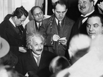
Myths are also rife. For instance, in the early twentieth century, when the theory’s founders were arguing among themselves about what it all meant, the views of Danish physicist Niels Bohr came to dominate. Albert Einstein famously disagreed with him and, in the 1920s and 1930s, the two locked horns in debate. A persistent myth was created that suggests Bohr won the argument by browbeating the stubborn and increasingly isolated Einstein into submission. Acting like some fanatical priesthood, physicists of Bohr’s ‘church’ sought to shut down further debate. They established the ‘Copenhagen interpretation’, named after the location of Bohr’s institute, as a dogmatic orthodoxy.
My latest book Quantum Drama, co-written with science historian John Heilbron, explores the origins of this myth and its role in motivating the singular personalities that would go on to challenge it. Their persistence in the face of widespread indifference paid off, because they helped to lay the foundations for a quantum-computing industry expected to be worth tens of billions by 2040.
John died on 5 November 2023, so sadly did not see his last work through to publication. This essay is dedicated to his memory.
Foundational myth
A scientific myth is not produced by accident or error. It requires effort. “To qualify as a myth, a false claim should be persistent and widespread,” Heilbron said in a 2014 conference talk. “It should have a plausible and assignable reason for its endurance, and immediate cultural relevance,” he noted. “Although erroneous or fabulous, such myths are not entirely wrong, and their exaggerations bring out aspects of a situation, relationship or project that might otherwise be ignored.”
Does quantum theory imply the entire Universe is preordained?
To see how these observations apply to the historical development of quantum mechanics, let’s look more closely at the Bohr–Einstein debate. The only way to make sense of the theory, Bohr argued in 1927, was to accept his principle of complementarity. Physicists have no choice but to describe quantum experiments and their results using wholly incompatible, yet complementary, concepts borrowed from classical physics.
In one kind of experiment, an electron, for example, behaves like a classical wave. In another, it behaves like a classical particle. Physicists can observe only one type of behaviour at a time, because there is no experiment that can be devised that could show both behaviours at once.
Bohr insisted that there is no contradiction in complementarity, because the use of these classical concepts is purely symbolic. This was not about whether electrons are really waves or particles. It was about accepting that physicists can never know what an electron really is and that they must reach for symbolic descriptions of waves and particles as appropriate. With these restrictions, Bohr regarded the theory to be complete — no further elaboration was necessary.
Such a pronouncement prompts an important question. What is the purpose of physics? Is its main goal to gain ever-more-detailed descriptions and control of phenomena, regardless of whether physicists can understand these descriptions? Or, rather, is it a continuing search for deeper and deeper insights into the nature of physical reality?
Einstein preferred the second answer, and refused to accept that complementarity could be the last word on the subject. In his debate with Bohr, he devised a series of elaborate thought experiments, in which he sought to demonstrate the theory’s inconsistencies and ambiguities, and its incompleteness. These were intended to highlight matters of principle; they were not meant to be taken literally.
Entangled probabilities
In 1935, Einstein’s criticisms found their focus in a paper1 published with his colleagues Boris Podolsky and Nathan Rosen at the Institute for Advanced Studies in Princeton, New Jersey. In their thought experiment (known as EPR, the authors’ initials), a pair of particles (A and B) interact and move apart. Suppose each particle can possess, with equal probability, one of two quantum properties, which for simplicity I will call ‘up’ and ‘down’, measured in relation to some instrument setting. Assuming their properties are correlated by a physical law, if A is measured to be ‘up’, B must be ‘down’, and vice versa. The Austrian physicist Erwin Schrödinger invented the term entangled to describe this kind of situation.
How Einstein built on the past to make his breakthroughs
If the entangled particles are allowed to move so far apart that they can no longer affect one another, physicists might say that they are no longer in ‘causal contact’. Quantum mechanics predicts that scientists should still be able to measure A and thereby — with certainty — infer the correlated property of B.
But the theory gives us only probabilities. We have no way of knowing in advance what result we will get for A. If A is found to be ‘down’, how does the distant, causally disconnected B ‘know’ how to correlate with its entangled partner and give the result ‘up’? The particles cannot break the correlation, because this would break the physical law that created it.
Physicists could simply assume that, when far enough apart, the particles are separate and distinct, or ‘locally real’, each possessing properties that were fixed at the moment of their interaction. Suppose A sets off towards a measuring instrument carrying the property ‘up’. A devious experimenter is perfectly at liberty to change the instrument setting so that when A arrives, it is now measured to be ‘down’. How, then, is the correlation established? Do the particles somehow remain in contact, sending messages to each other or exerting influences on each other over vast distances at speeds faster than light, in conflict with Einstein’s special theory of relativity?
The alternative possibility, equally discomforting to contemplate, is that the entangled particles do not actually exist independently of each other. They are ‘non-local’, implying that their properties are not fixed until a measurement is made on one of them.
Both these alternatives were unacceptable to Einstein, leading him to conclude that quantum mechanics cannot be complete.
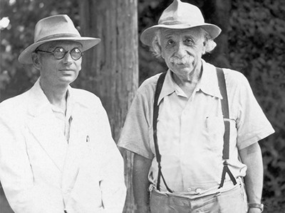
Niels Bohr (left) and Albert Einstein.Credit: Universal History Archive/Universal Images Group via Getty
The EPR thought experiment delivered a shock to Bohr’s camp, but it was quickly (if unconvincingly) rebuffed by Bohr. Einstein’s challenge was not enough; he was content to criticize the theory but there was no consensus on an alternative to Bohr’s complementarity. Bohr was judged by the wider scientific community to have won the debate and, by the early 1950s, Einstein’s star was waning.
Unlike Bohr, Einstein had established no school of his own. He had rather retreated into his own mind, in vain pursuit of a theory that would unify electromagnetism and gravity, and so eliminate the need for quantum mechanics altogether. He referred to himself as a “lone traveler”. In 1948, US theoretical physicist J. Robert Oppenheimer remarked to a reporter at Time magazine that the older Einstein had become “a landmark, but not a beacon”.
Prevailing view
Subsequent readings of this period in quantum history promoted a persistent and widespread suggestion that the Copenhagen interpretation had been established as the orthodox view. I offer two anecdotes as illustration. When learning quantum mechanics as a graduate student at Harvard University in the 1950s, US physicist N. David Mermin recalled vivid memories of the responses that his conceptual enquiries elicited from his professors, whom he viewed as ‘agents of Copenhagen’. “You’ll never get a PhD if you allow yourself to be distracted by such frivolities,” they advised him, “so get back to serious business and produce some results. Shut up, in other words, and calculate.”
The spy who flunked it: Kurt Gödel’s forgotten part in the atom-bomb story
It seemed that dissidents faced serious repercussions. When US physicist John Clauser — a pioneer of experimental tests of quantum mechanics in the early 1970s — struggled to find an academic position, he was clear in his own mind about the reasons. He thought he had fallen foul of the ‘religion’ fostered by Bohr and the Copenhagen church: “Any physicist who openly criticized or even seriously questioned these foundations … was immediately branded as a ‘quack’. Quacks naturally found it difficult to find decent jobs within the profession.”
But pulling on the historical threads suggests a different explanation for both Mermin’s and Clauser’s struggles. Because there was no viable alternative to complementarity, those writing the first post-war student textbooks on quantum mechanics in the late 1940s had little choice but to present (often garbled) versions of Bohr’s theory. Bohr was notoriously vague and more than occasionally incomprehensible. Awkward questions about the theory’s foundations were typically given short shrift. It was more important for students to learn how to apply the theory than to fret about what it meant.
One important exception is US physicist David Bohm’s 1951 book Quantum Theory, which contains an extensive discussion of the theory’s interpretation, including EPR’s challenge. But, at the time, Bohm stuck to Bohr’s mantra.
The Americanization of post-war physics meant that no value was placed on ‘philosophical’ debates that did not yield practical results. The task of ‘getting to the numbers’ meant that there was no time or inclination for the kind of pointless discussion in which Bohr and Einstein had indulged. Pragmatism prevailed. Physicists encouraged their students to choose research topics that were likely to provide them with a suitable grounding for an academic career, or ones that appealed to prospective employers. These did not include research on quantum foundations.
These developments conspired to produce a subtly different kind of orthodoxy. In The Structure of Scientific Revolutions (1962), US philosopher Thomas Kuhn describes ‘normal’ science as the everyday puzzle-solving activities of scientists in the context of a prevailing ‘paradigm’. This can be interpreted as the foundational framework on which scientific understanding is based. Kuhn argued that researchers pursuing normal science tend to accept foundational theories without question and seek to solve problems within the bounds of these concepts. Only when intractable problems accumulate and the situation becomes intolerable might the paradigm ‘shift’, in a process that Kuhn likened to a political revolution.
Do black holes explode? The 50-year-old puzzle that challenges quantum physics
The prevailing view also defines what kinds of problem the community will accept as scientific and which problems researchers are encouraged (and funded) to investigate. As Kuhn acknowledged in his book: “Other problems, including many that had previously been standard, are rejected as metaphysical, as the concern of another discipline, or sometimes as just too problematic to be worth the time.”
What Kuhn says about normal science can be applied to ‘mainstream’ physics. By the 1950s, the physics community had become broadly indifferent to foundational questions that lay outside the mainstream. Such questions were judged to belong in a philosophy class, and there was no place for philosophy in physics. Mermin’s professors were not, as he had first thought, ‘agents of Copenhagen’. As he later told me, his professors “had no interest in understanding Bohr, and thought that Einstein’s distaste for [quantum mechanics] was just silly”. Instead, they were “just indifferent to philosophy. Full stop. Quantum mechanics worked. Why worry about what it meant?”
It is more likely that Clauser fell foul of the orthodoxy of mainstream physics. His experimental tests of quantum mechanics2 in 1972 were met with indifference or, more actively, dismissal as junk or fringe science. After all, as expected, quantum mechanics passed Clauser’s tests and arguably nothing new was discovered. Clauser failed to get an academic position not because he had had the audacity to challenge the Copenhagen interpretation; his audacity was in challenging the mainstream. As a colleague told Clauser later, physics faculty members at one university to which he had applied “thought that the whole field was controversial”.
Aspect, Clauser and Zeilinger won the 2022 physics Nobel for work on entangled photons.Credit: Claudio Bresciani/TT News Agency/AFP via Getty
However, it’s important to acknowledge that the enduring myth of the Copenhagen interpretation contains grains of truth, too. Bohr had a strong and domineering personality. He wanted to be associated with quantum theory in much the same way that Einstein is associated with theories of relativity. Complementarity was accepted as the last word on the subject by the physicists of Bohr’s school. Most vociferous were Bohr’s ‘bulldog’ Léon Rosenfeld, Wolfgang Pauli and Werner Heisenberg, although all came to hold distinct views about what the interpretation actually meant.
They did seek to shut down rivals. French physicist Louis de Broglie’s ‘pilot wave’ interpretation, which restores causality and determinism in a theory in which real particles are guided by a real wave, was shot down by Pauli in 1927. Some 30 years later, US physicist Hugh Everett’s relative state or many-worlds interpretation was dismissed, as Rosenfeld later described, as “hopelessly wrong ideas”. Rosenfeld added that Everett “was undescribably stupid and could not understand the simplest things in quantum mechanics”.
Unorthodox interpretations
But the myth of the Copenhagen interpretation served an important purpose. It motivated a project that might otherwise have been ignored. Einstein liked Bohm’s Quantum Theory and asked to see him in Princeton in the spring of 1951. Their discussion prompted Bohm to abandon Bohr’s views, and he went on to reinvent de Broglie’s pilot wave theory. He also developed an alternative to the EPR challenge that held the promise of translation into a real experiment.
Befuddled by Bohrian vagueness, finding no solace in student textbooks and inspired by Bohm, Irish physicist John Bell pushed back against the Copenhagen interpretation and, in 1964, built on Bohm’s version of EPR to develop a now-famous theorem3. The assumption that the entangled particles A and B are locally real leads to predictions that are incompatible with those of quantum mechanics. This was no longer a matter for philosophers alone: this was about real physics.
It took Clauser three attempts to pass his graduate course on advanced quantum mechanics at Columbia University because his brain “kind of refused to do it”. He blamed Bohr and Copenhagen, found Bohm and Bell, and in 1972 became the first to perform experimental tests of Bell’s theorem with entangled photons2.
How to introduce quantum computers without slowing economic growth
French physicist Alain Aspect similarly struggled to discern a “physical world behind the mathematics”, was perplexed by complementarity (“Bohr is impossible to understand”) and found Bell. In 1982, he performed what would become an iconic test of Bell’s theorem4, changing the settings of the instruments used to measure the properties of pairs of entangled photons while the particles were mid-flight. This prevented the photons from somehow conspiring to correlate themselves through messages or influences passed between them, because the nature of the measurements to be made on them was not set until they were already too far apart. All these tests settled in favour of quantum mechanics and non-locality.
Although the wider physics community still considered testing quantum mechanics to be a fringe science and mostly a waste of time, exposing a hitherto unsuspected phenomenon — quantum entanglement and non-locality — was not. Aspect’s cause was aided by US physicist Richard Feynman, who in 1981 had published his own version of Bell’s theorem5 and had speculated on the possibility of building a quantum computer. In 1984, Charles Bennett at IBM and Giles Brassard at the University of Montreal in Canada proposed entanglement as the basis for an innovative system of quantum cryptography6.
It is tempting to think that these developments finally helped to bring work on quantum foundations into mainstream physics, making it respectable. Not so. According to Austrian physicist Anton Zeilinger, who has helped to found the science of quantum information and its promise of a quantum technology, even those working in quantum information consider foundations to be “not the right thing”. “We don’t understand the reason why. Must be psychological reasons, something like that, something very deep,” Zeilinger says. The lack of any kind of physical mechanism to explain how entanglement works does not prevent the pragmatic physicist from getting to the numbers.
Similarly, by awarding the 2022 Nobel Prize in Physics to Clauser, Aspect and Zeilinger, the Nobels as an institution have not necessarily become friendly to foundational research. Commenting on the award, the chair of the Nobel Committee for Physics, Anders Irbäck, said: “It has become increasingly clear that a new kind of quantum technology is emerging. We can see that the laureates’ work with entangled states is of great importance, even beyond the fundamental questions about the interpretation of quantum mechanics.” Or, rather, their work is of great importance because of the efforts of those few dissidents, such as Bohm and Bell, who were prepared to resist the orthodoxy of mainstream physics, which they interpreted as the enduring myth of the Copenhagen interpretation.
The lesson from Bohr–Einstein and the riddle of entanglement is this. Even if we are prepared to acknowledge the myth, we still need to exercise care. Heilbron warned against wanton slaying: “The myth you slay today may contain a truth you need tomorrow.”
A high-end wireless gaming headset designed for Xbox, the JBL Quantum 910X falls just short of earning a place among the best Xbox Series X headsets. That’s not to say that it isn’t still a formidable option, however, as it offers an excellent level of comfort that’s backed up by rich audio; it’s absolutely perfect for many of the best Xbox Series X games. In addition to Xbox, it’s also fully compatible with PlayStation, Nintendo Switch, and PC, making it a strong multi-platform choice.
Unfortunately, the flagship feature of the JBL Quantum 910X, its head-tracking 360 degree spatial audio, is a mixed bag. The head-tracking itself is exceptional, simulating your head motion perfectly, but the audio quality takes a substantial hit whenever the feature is enabled. The bass becomes almost non-existent, completely ruining the punchy action of first-person shooter (FPS) titles like Call of Duty: Modern Warfare 3, while the high end frequencies sound sharp and unpleasant. If your number one concern is high-quality spatial sound, no shortage of cheaper headsets like the SteelSeries Arctis Nova 7X, offer far superior spatial audio.
The microphone is the only other major area where the JBL Quantum 910X falls behind the competition. It lacks adjustability and leaves your voice sounding grainy and quiet. It’s by no means unusable, but this is nowhere near the level of performance that you would reasonably expect for this price. Whether this is the headset for you is therefore going to depend on whether these two shortcomings are a total deal breaker but, if they’re not, there’s still an awful lot to like here.
(Image credit: Dashiell Wood / Future)
Price and availability
$299.95 / £219.99
Available in the US and UK
Better value in the UK
The JBL Quantum 910X costs $299.95 / £219.99 and is available in the US and UK directly from JBL or at retailers like Amazon. In the US, this comes in slightly cheaper than other high-end gaming headsets, such as the $329.99 / £279.99 Turtle Beach Stealth Pro, but is still firmly in premium territory. All things considered, it’s quite a reasonable price when you factor in the presence of high-end features such as active noise cancellation, not to mention customizable RGB lighting and the robust build quality.
Even so, UK price represents the best value of the two regions. At £219.99, the headset is a massive £60 less expensive than the Turtle Beach Stealth Pro, widening the gap between the two headsets and making the JBL Quantum 910X a much more tempting proposition.
Unfortunately, the JBL Quantum 910X is not currently available in Australia.
Specs
Swipe to scroll horizontally
Price
$299.95 / £219.99
Weight
14.8 oz / 420g
Quoted battery life
37 hours
Features
Active noise cancellation, JBL QuantumSpatial 360 head-tracking spatial audio
Connection type
Wireless (USB-C dongle), wired (USB-C / 3.5mm)
Compatibility
Xbox Series X, Xbox Series S, Xbox One, PlayStation 5, PlayStation 4, PC, Nintendo Switch, Android, iOS
Software
JBL Quantum Engine (PC)
(Image credit: Dashiell Wood / Future)
Design and features
The exterior of the JBL Quantum 910X is primarily constructed from a smooth black plastic. Its ear cups are covered in bright RGB lighting, illuminating in a ring around each ear in addition to an area with a small grill-like pattern and a prominent embossed JBL logo. The lighting is set to green by default which is perfect if you intend to use the headset with an Xbox out of the box. This lighting can be fully customized through the compatible JBL Quantum Engine software on a PC.
Each ear cup is connected to the headband with a clear plastic strip and a short braided cable, which is black with subtle green stripes. The clear plastic portion can be extended or retracted in order to customize the fit, engraved with numbers that indicate different sizing settings. The ear cups themselves then use soft black pleather cushions, which are a generous size and pleasantly soft.
The same cushioning is also found on the underside of the headband itself, which is topped with black plastic covered in a tactile grooved design. Although the JBL Quantum 910X is notably heavier than many other gaming headsets, weighing a hefty 14.8oz / 420g, the comfortable cushions makes it surprisingly easy to wear for extended periods without discomfort.
(Image credit: Dashiell Wood / Future)
The microphone is attached to the left ear cup and can be raised or lowered. It’s muted by default in its raised position, indicated by a small red LED light near its tip. There’s also a separate dedicated microphone mute button on the back of the ear cup, which is handy if you want to quickly mute the microphone without having to raise it. This is positioned below a volume dial, a volume mixer dial (which changes the balance between in-game audio and audio from a connected mobile phone), and a switch which enables or disables the headset’s active noise cancellation. On the bottom of the left ear cup you will also find the USB Type-C port, which can be used for both charging and wired play. It’s next to a 3.5mm headphone jack and superb braided cables for both are included in the box.
Controls on the right ear cup are simpler, with a power slider that doubles as a switch to enable Bluetooth connectivity and a simple button that alternates between standard audio, spatial sound, and full head-tracking. Although it can be used out of the box, spatial sound can be further calibrated for enhanced precision in the JBL Quantum Engine software.
This is a simple process with clear on screen instructions, but does require an included detachable microphone to sit in your ear. Factor in the wireless dongle, which comes alongside a compact USB Type-A to USB Type-C converter and that’s a lot of separate accessories to keep track of. Luckily, the headset comes with an absolutely lovely plush gray bag which is perfect for keeping everything in one place.
(Image credit: Dashiell Wood / Future)
Performance
In its standard mode, the JBL Quantum 910X performs excellently on the whole. It offers punchy, rich bass, clear mids, and detailed high-end frequencies. While its overall audio profile might be a little too bass-heavy for audiophile music listening, it’s absolutely perfect for gaming and the range of titles I tested sounded superb. Shots in Call of Duty: Modern Warfare 3 packed some serious punch on Xbox Series S, while the streets of Sotenbori in the PC version of Like a Dragon Gaiden: The Man Who Erased His Namefelt impressively life-like.
The emphasis on bass is also an excellent fit for rhythm games and I enjoyed quite a bit of success challenging myself with “JITTERBUG” on Extreme difficulty in Hatsune Miku: Project DIVA Future Tone on PS5. The JBL Quantum Engine software offers a range of useful equalizer modes and is, on the whole, some of the best companion software that I’ve ever tested. It offers an impressive number of functions, features an intuitive and attractive UI, and is lightning fast while taking up just 255MB of space. A mobile app or a native application for Xbox would enable those without access to a PC to benefit from its features, but otherwise there is nothing to complain about here.
(Image credit: JBL)
Returning to the headset, the on-board controls are well-spaced and responsive, while the active noise cancellation is a treat. It’s very effective and managed to block out almost everything that I could throw at it, ranging all the way from nearby conversations to loud passing vehicles. I also consistently managed to squeeze an impressive 32 hours of battery life out of the headset, which was more than enough for a full week of gaming sessions.
Unfortunately, the performance with the spatial audio mode enabled is a completely different story. The illusion of depth is there, but the bass instantly vanishes leading to an incredibly tinny sound that lacks any impact whatsoever. It’s like listening to a tiny pair of cheap speakers in a massive hall, an impression that is only further reinforced by the oddly echoey sound of any dialogue.
The optional head tracking, which sees the audio source shift as you look around, is incredibly accurate and well worth experimenting with for a few minutes, but the dramatic fall in audio quality means that it’s impossible to recommend using the spatial audio mode for any substantial length of time which is a huge shame.
The microphone performance is also disappointing. The physical microphone itself is unusually rigid and cannot be adjusted to be closer or further away from your mouth very easily. I found that this meant that my voice often sounded rather quiet and a little muddy. I was still easy to understand, once every participant of my calls had adjusted their volume accordingly, but this really shouldn’t be necessary with such an expensive peripheral.
(Image credit: Dashiell Wood / Future)
Should I buy the JBL Quantum 910X?
Buy it if…
Don’t buy it if…
Also consider
If you’re not keen on the JBL Quantum 910X, you should consider these two compelling Xbox-compatible alternatives instead.
Xbox Series X, Xbox Series S, Xbox One, PlayStation 5, PlayStation 4, PC, Nintendo Switch, Android, iOS
Xbox Series X, Xbox Series S, Xbox One, PlayStation 5, PlayStation 4, PC, Nintendo Switch, Android, iOS
Xbox Series X, Xbox Series S, Xbox One, PlayStation 5, PlayStation 4, PC, Nintendo Switch, Android, iOS
Software
JBL Quantum Engine (PC)
Turtle Beach Audio Hub (PC / Android / iOS))
SteelSeries Sonar (PC)
How I tested the JBL Quantum 910X
Used daily for over a month
Tested with a wide range of platforms
Compared to other premium gaming headsets
I tested the JBL Quantum 910X for over a month, using it as my main gaming headset. During that time, I tested the headset with Xbox Series S, PlayStation 5, PC, and Nintendo Switch playing a broad range of titles. In addition to my usual favorites, I tried to focus on some modern games that offer rich sound, including the likes of Counter-Strike 2, Need for Speed Unbound, The Last of Us Part 2 Remastered, and Fortnite. In order to test the microphone, I used the headset for multiple online gaming sessions and recorded a number of audio files with Audacity.
Throughout my time with the headset, I was careful to compare the experience with my hands-on time with other high-end gaming headsets such as the SteelSeries Arctis Nova 7X, Astro A50 X, and Turtle Beach Stealth Pro .
Unlike traditional computing that uses binary bits, quantum computing uses quantum bits or ‘qubits’, enabling simultaneous processing of vast amounts of data, potentially solving complex problems much faster than conventional computers.
In a major step forward for quantum computing, Microsoft and Quantinuum have unveiled the most reliable logical qubits to date, boasting an error rate 800 times lower than physical qubits.
This groundbreaking achievement involved running over 14,000 individual experiments without a single error, which could make quantum computing a viable technology for various industries.
Azure Quantum Elements platform
Microsoft says the successful demonstration was made possible by applying its innovative qubit-virtualization system (coupled with error diagnostics and correction) to Quantinuum’s ion-trap hardware. Jason Zander, EVP of Strategic Missions and Technologies at Microsoft, says, “This finally moves us out of the current noisy intermediate-scale quantum (NISQ) level to Level 2 Resilient quantum computing.”
The potential of this advancement is enormous. As Zander says, “With a hybrid supercomputer powered by 100 reliable logical qubits, organizations would start to see the scientific advantage, while scaling closer to 1,000 reliable logical qubits would unlock commercial advantage.”
Quantum computing holds enormous promise for solving some of society’s most daunting challenges, including climate change, food shortages, and the energy crisis. These issues often boil down to complex chemistry and materials science problems, which classical computing struggles to handle but which would be far easier for Quantum computers to manage.
The task now, Microsoft says, is to continue improving the fidelity of qubits and enable fault-tolerant quantum computing. This will involve transitioning to reliable logical qubits, a feat achieved by merging multiple physical qubits to protect against noise and sustain resilient computation.
Sign up to the TechRadar Pro newsletter to get all the top news, opinion, features and guidance your business needs to succeed!
While the technology’s potential is immense, its widespread adoption will depend on its accessibility and cost-effectiveness. For now, though, Microsoft and Quantinuum’s breakthrough marks a significant step towards making quantum computing a practical reality.
While classical computers and electronics rely on binary bits as their basic unit of information (they can be either on or off), quantum computers work with qubits, which can exist in a superposition of two states at the same time. The trouble with qubits is that they’re prone to error, which is the main reason today’s quantum computers (known as Noisy Intermediate Scale Quantum [NISQ] computers) are just used for research and experimentation.
Microsoft’s solution was to group physical qubits into virtual qubits, which allows it to apply error diagnostics and correction without destroying them, and run it all over Quantinuum’s hardware. The result was an error rate that was 800 times better than relying on physical qubits alone. Microsoft claims it was able to run more than 14,000 experiments without any errors.
According to Jason Zander, EVP of Microsoft’s Strategic Missions and Technologies division, this achievement could finally bring us to “Level 2 Resilient” quantum computing, which would be reliable enough for practical applications.
“The task at hand for the entire quantum ecosystem is to increase the fidelity of qubits and enable fault-tolerant quantum computing so that we can use a quantum machine to unlock solutions to previously intractable problems,” Zander, wrote in a blog post today. “In short, we need to transition to reliable logical qubits — created by combining multiple physical qubits together into logical ones to protect against noise and sustain a long (i.e., resilient) computation. … By having high-quality hardware components and breakthrough error-handling capabilities designed for that machine, we can get better results than any individual component could give us.”
Microsoft
Researchers will be able to get a taste of Microsoft’s reliable quantum computing via Azure Quantum Elements in the next few months, where it will be available as a private preview. The goal is to push even further to Level 3 quantum supercomputing, which will theoretically be able to tackle incredibly complex issues like climate change and exotic drug research. It’s unclear how long it’ll take to actually reach that point, but for now, at least we’re moving one step closer towards practical quantum computing.
This article contains affiliate links; if you click such a link and make a purchase, we may earn a commission.
To experimentally realize a curved spacetime such as a black hole requires a specific relative motion between the excitations and the background medium. One-dimensional supersonic flow, the archetypal example of an acoustic black hole, provides a platform for observations of Hawking radiation in both classical20,21 and quantum fluids9,10,22. More complex phenomena such as Penrose superradiance require rotating geometries realizable in two spatial dimensions, for example, by means of a stationary draining vortex flow12,23. Classical fluid flow experiments have demonstrated the power of the gravity simulator programme, realizing superradiant amplification of both coherent11,24 and evanescent waves25, as well as quasinormal mode oscillations26, a process intimately connected to black hole ringdown27.
Here we investigate related phenomena in the limit of negligible viscosity in superfluid 4He (called He II). Its energy dissipation is dependent on temperature and can be finely adjusted across a wide range. At 1.95 K, at which our experiments take place, its kinematic viscosity is reduced by a factor of 100 compared with water28 and the damping is dominated by thermal excitations collectively described by the viscous normal component28,29 that constitutes approximately half of the total density of the liquid. Moreover, He II supports the existence of line-like topological defects called quantum vortices. Each vortex carries a single circulation quantum κ ≈ 10−7 m2 s−1 and forms an irrotational (zero-curl) flow field in its vicinity29. Owing to this discretization, a draining vortex of He II can manifest itself only as a multiply quantized (also known as giant) vortex or as a cluster of single quantum vortices. Such vortex bundles exhibit their own collective dynamics and can even introduce solid-body rotation30 at length scales larger than the inter-vortex distance, adding complexity to the study of quantum fluid behaviour. As the realization of curved spacetime scenarios requires an irrotational velocity field1,31, it is critical to confine any rotational elements into a central area, that is, the vortex core. However, alike-oriented vortices have a tendency to move apart from each other, which poses a limitation on the extent of the core one can stabilize in an experiment. On the other hand, recent findings show that mutual friction29 between quantum vortices and the normal component contributes to the stabilization of dense vortex clusters32.
The vortex induces a specific velocity field within the superfluid, which affects the propagation of small waves on its surface. In particular, low-frequency excitations perceive an effective acoustic metric3,4
in which c denotes their propagation speed and \({\bf{v}}(r,\theta )={v}_{r}\widehat{{\bf{r}}}+{v}_{\theta }\widehat{{\boldsymbol{\theta }}}\) indicates the velocity field at the interface (we assume that the superfluid and normal velocity fields are equal, in line with other mechanically driven flows of He II (refs. 33,34)). Although this description fails in the high-frequency regime owing to dispersion, it is well known that the curved spacetime phenomenology persists for these excitations24,26,35. Altogether, the above properties suggest that an extensive draining vortex of He II is a feasible candidate for simulations of a quantum field theory in curved spacetime.
We realized this flow in cylindrical geometry that is built on the concept of a stationary suction vortex36 (see Methods for a detailed description). The central component of our set-up is a spinning propeller, which is responsible for establishing a continuous circulating loop of He II, feeding a draining vortex that forms in the optically accessible experimental zone. At small propeller speeds, we observe a depression on the superfluid interface (Fig. 1a), but as the speed increases, this depression deepens and eventually transforms into a hollow vortex core extending from the free surface to the bottom drain (Fig. 1b). The parabolic shape of the free surface in the former regime is consistent with solid-body rotation, which corresponds to a compact, polarized cluster of singly quantized vortices (called solid core) that forms under the finite depression. The hollow core can instead absorb individual circulation quanta and behave like a multiply quantized object37. To minimize the rotational flow injected by the spinning propeller into the experimental zone, we devised a unique recirculation strategy based on a purpose-built flow conditioner (see Methods) that promotes formation of a centrally confined vortex cluster instead of a sparse vortex lattice. However, the exact dynamics of individual quantum vortices, as well as their spatial distribution in the experiment, calls for future investigations. State-of-the-art numerical models38 account for the motion of vortex lines coupled to the superfluid and normal velocity fields, but fail to dynamically model the interface, which is a pivotal element in our system. Previous experimental efforts39,40,41 confirmed that a draining vortex in He II carries macroscopic circulation but lacked spatial resolution required to investigate central confinement of rotational components. In this regard, cryogenic flow visualization42 provides sufficient resolution. However, this method requires introducing small solid particles into the superfluid, which accumulate along the vortex lines and considerably affect their dynamics43.
Fig. 1: Side views of two distinct configurations of the giant quantum vortex.
a, At low propeller frequencies (here 1 Hz), the interface exhibits a discernible depression, and the vortex core beneath takes the form of a compact, polarized cluster of singly quantized vortices (called solid core). b, With the escalation of frequency (here to 2 Hz), a fully formed hollow core emerges, behaving like a multiply quantized object. Dark vertical stripes in the background provide contrast to the imaged interface. A simplified sketch of this interface (white lines) helps to identify these regimes in later figures. Scale bar, 10 mm.
The above limitations compelled us to propose an alternative, minimally invasive method to examine the vortex flow and extract macroscopic flow parameters that exploit the relative motion occurring between interface waves and the underlying velocity field. The corresponding dispersion relation for angular frequencies ω and wave vectors k reads35
in which F denotes the dispersion function. By solving equation (2), we find (see Methods) that the spectrum of interface modes gets frequency shifted and the velocity field can be inferred from these shifts44. Therefore, we redirect our attention towards precise detection of small waves propagating on the superfluid interface.
We identified that the adapted Fourier transform profilometry17,18 is well suited to our needs, as it is capable of resolving a fluid interface with sufficient and simultaneous resolution in both space and time. This powerful technique consists of imaging the disturbed interface against a periodic backdrop pattern. This way, we resolve height fluctuations of said interface (Fig. 2a) with sensitivity up to approximately one micrometre. Owing to symmetries of the flow, the waves exhibit two conserved quantities: frequency f and azimuthal number m. The latter parameter counts the number of wave crests around a circular path, with positive or negative values of m corresponding to wave patterns co-rotating or counter-rotating with the central vortex.
Fig. 2: Superfluid interface reconstruction and wave analysis.
a, Snapshot of the free helium surface depicts height fluctuations representing micrometre waves excited on the superfluid interface. Grey areas mark the positions of the central drain (radius 5 mm) and the outer glass wall (radius 37.3 mm). b–e, Examples of different azimuthal modes |m| (m counting the number of wave crests or troughs around a circular path) extracted from panel a by a discrete Fourier transform. Wave amplitudes are rescaled for better visibility. f,g, Two-dimensional wave spectra obtained by transforming angle and time coordinates, for radii of 11.2 mm (panel f) and 22.1 mm (panel g). These radii are marked in panel a by coloured circles. Absence of excitations in low-frequency bands (below the coloured lines) can be understood through the solution of equation (2). The corresponding theoretical predictions of the minimum frequency permissible for propagation for the given radii can be matched with experimental observations (yellow and red lines).
These spatial patterns (or modes) can be retrieved from the height-fluctuation field by a discrete Fourier transform. For example, by transforming with respect to the angle θ, we can single out individual azimuthal modes (Fig. 2b–e). To study wave dynamics in time, we must also transform the temporal coordinate and inspect the resulting two-dimensional spectra, showcased in Fig. 2f,g for two distinct radii. Notable high-amplitude signals in the m = ±1 bands are exclusively a consequence of how mechanical vibrations of the set-up imprint themselves on our detection method. Of physical interest are modes with higher azimuthal numbers. These excitations, observed in both solid-core and hollow-core regimes, represent micrometre waves excited on the interface. In the steady state, the waves dissipate their energy, in part by viscous damping and in part by scattering into the draining core of the vortex45. Although this is balanced by the stochastic drive originating from the fluid flow and/or aforementioned mechanical vibrations, we notice that only a certain region of the spectral space (m, f) is populated with excitations, a feature that varies when examining smaller (Fig. 2f) and larger (Fig. 2g) radii. We observe that only some high-frequency (equivalent to high-energy) waves have the capability to propagate on the interface. Through the solution of equation (2), we can pinpoint the minimum frequency, fmin, permissible for propagation for the given radius, azimuthal number and background velocity (see Methods) and, in line with the methodology introduced above, we exploit this particular frequency to extract the underlying velocity field, as we now describe. We search the parameter space produced by two velocity components (vr, vθ) and determine values that produce the best match between fmin and the lowest excited frequency in the experimental data across several azimuthal modes (coloured lines in Fig. 2f,g). By carrying out this procedure for every examined radius, we can reconstruct the velocity distribution in the draining vortex flow.
We conducted these reconstructions across several vortex configurations distinguished by the drive (propeller) frequency. For all instances, vr approximates zero within the limits of our resolution. Although seemingly paradoxical, this outcome results from a complex boundary-layer interaction and is in agreement with earlier findings in classical fluids46. Therefore, interface waves engage with an almost entirely circulating flow characterized by a specific radial dependence of vθ (coloured points in Fig. 3a). Overall, the results are consistent with
$${v}_{\theta }(r)=\varOmega r+\frac{C}{r},$$
(3)
indicated in Fig. 3a by coloured lines. The first term represents solid-body rotation with angular frequency Ω, which leaks into the experimental area through the flow conditioner as described above. The second term corresponds to an irrotational flow around a central vortex with circulation C. The related number of circulation quanta confined in its core, NC = 2πC/κ, is shown in Fig. 3b as a function of the drive frequency. Across all instances, the core consists of the order of 104 quanta, a record-breaking value in the realm of quantum fluids. In the solid-core regime, NC can be identified with the number of individual quantum vortices concentrated in the core. However, in the context of a hollow core, NC represents its topological charge. Achieving circulation values separated from the elementary quantum κ by four orders of magnitude allows the quantization of circulation to be disregarded, leaving the vortex effectively classical. This unprecedented realization of a giant quantum vortex flow represents a distinctive instance of a quantum-to-classical flow transition in He II (ref. 47).
Fig. 3: Reconstructed velocity distribution and flow parameters.
a, Coloured points denote the radial dependence of the azimuthal velocity vθ for six vortex configurations distinguished by the drive (propeller) frequency. Each point is obtained by averaging over a 2.5-mm radial interval. Radial velocity component is approximately zero across all instances. Best fits of vθ(r) (coloured lines) yield the circulation C of the central vortex and the angular frequency Ω of the extra solid-body rotation. b, Number of circulation quanta confined in the vortex core, NC = 2πC/κ, corresponds to the most extensive vortex structures ever observed in quantum fluids. c, The ratio η between Ω and the angular frequency of the drive is less than 2.5% in all cases, suggesting that the velocity field in our system is dominated by the irrotational vortex flow. Vertical error bars in panels a and c denote one standard deviation intervals. Standard deviation intervals of data points in panel b, comparable with the symbol size, are not shown.
The importance of the aforementioned outcomes can be underlined by noting that n-quantized vortices are dynamically unstable13,14. They spontaneously decay into a cluster of n vortices48 as a result of the excitation of a negative energy mode in the multiply quantized vortex core11,48. Nevertheless, dynamical stabilization of giant vortices can be achieved by suitably manipulating the superfluid. Namely, introducing a draining flow and reducing the fluid density at the centre has proven effective in polariton condensates, for vortices with n≲ 100 (refs. 15,16). These results agree with our experiment, in which the reduced density translates into the existence of a hollow core and the draining flow resides in the bulk of the draining vortex.
It is worth noting that larger circulation values around a draining vortex in He II are documented in the literature41. However, therein, the contributions of the vortex core and the solid-body rotation are not distinguished. The second effect may dominate in the reported circulations, as the number of quantum vortices responsible for rotation30 scales with the corresponding angular frequency Ω. Rotation in our experimental zone is notably suppressed. The sparse presence of quantum vortices partially justifies our assumption that normal and superfluid components behave as a single fluid. More importantly, the ratio η between Ω and the angular frequency of the drive does not exceed 2.5% (Fig. 3c), and the velocity field in our system is dominated by the irrotational vortex flow. The core of this vortex must be smaller than 7.6 mm, the smallest investigated radius, because the velocity profiles (Fig. 3a) show no indication of a turning point at small radii.
We can, nonetheless, venture beyond the experimental range by exploring wave dynamics in the radial direction. We restrict our discussion to a particular mode |m| = 8 (Fig. 2d) as a representative of the outlined behaviour. We start by analysing co-rotating (m = 8) modes, shown in Fig. 4a,b for the solid-core and hollow-core structures. In both cases, fmin (red line) denotes an effective potential barrier, preventing waves from reaching the vortex core. Existence of this barrier, together with an outer, solid boundary at 37.3 mm, gives rise to bound states (standing waves), appearing as distinct, striped patterns extending up to 40 Hz. These patterns represent the first direct measurement of resonant surface modes around a macroscopic vortex flow in He II.
Fig. 4: Bound states in co-rotating waves.
Fourier amplitudes of interface waves corresponding to m = 8 mode show a characteristic pattern in the radial direction that can be identified with bound states, that is, standing waves between the outer boundary (glass wall) at 37.3 mm and the effective potential barrier (red lines). A simplified but accurate model of the potential (yellow lines) is extended beyond the experimentally accessible range (dashed black lines). a, Solid-core regime. Rescaled amplitudes of four bound states labelled I–IV (blue lines) are shown as a function of radius. Crossing points with the potential barrier are marked by yellow points. b, Hollow-core regime. c, Comparison of bound-state frequencies retrieved from panel a (red points) and their theoretical predictions (black circles). Frequencies of states I–IV are highlighted by blue arrows.
To perform an in-depth examination of selected states (denoted as I–IV), we plot the absolute value of their amplitudes in Fig. 4a. The frequency of state I meets fmin in a crossing point (yellow point) located within the field of view. At large radii, this wave harmonically propagates. However, as it penetrates the barrier, its amplitude exponentially decays in exact analogy with a simple quantum-mechanical model of a particle trapped in a potential well. For higher frequencies, the crossing point moves towards smaller radii (state II), eventually reaching the limit of our detection range. For the highest-frequency states (III and IV), the crossing point is well outside the detection range and we only observe the harmonic part of the signal. Nonetheless, the mere existence and predictability of these states lets us extend the effective potential barrier beyond the observable range.
Specifically, we consider a model of a purely circulating vortex, whose velocity field reads (vr, vθ) = (0, C/r), and extend the experimentally determined potential barrier (red lines in Fig. 4a,b) towards smaller radii (yellow lines). In practice, this model must break down near the vortex core, at which point the spatial distribution of individual quantum vortices becomes relevant. Nonetheless, the frequencies of individual bound states are in excellent agreement with theoretical predictions (see Methods) based on the extended potential barrier (Fig. 4c). This outcome validates the simplified model and allows us to constrain the radius of the core region to approximately 4 and 6 mm, respectively for the solid-core and hollow-core regimes. Confinement of the rotating core beyond the experimental range gains importance when considering the draining vortex flow as a gravity simulator, for example, when searching for initial indications of black hole ringdown.
For this purpose, we focus on counter-rotating (m = −8) modes, depicted in Fig. 5a,b with the effective potential barriers (red lines) and their extensions (yellow lines). The shape of the barrier in the solid-core regime (Fig. 5a) allows the existence of bound states up to approximately 30 Hz. However, this is not the case in the hollow-core regime (Fig. 5b), despite the corresponding circulations only differing within one order of magnitude. Bound states are not formed at all because the effective potential shows a shallow maximum before decreasing towards zero. Dominant excitations in this spectrum, highlighted in Fig. 5c, are modes lingering near this maximum. These excitations, previously identified as ringdown modes of an analogue black hole26, represent the very first hints of this process taking place in a quantum fluid. The radius at which the effective potential crosses the zero-frequency level is related to the analogue ergoregion35, a key feature in the occurrence of black hole superradiance. To directly observe this region in our set-up, further increasing the azimuthal velocity and/or examining the system closer to the vortex core is required.
Fig. 5: Bound states and ringdown modes in counter-rotating waves.
Fourier amplitudes of interface waves (same colour scale as in Fig. 4) corresponding to m = −8 mode interact with the effective potential barrier (red lines). Its simplified model (yellow lines) is extended beyond the accessible range (dashed black lines). a, In the solid-core regime, the potential allows existence of bound states, visible up to approximately 30 Hz. b, In the hollow-core regime, no bound states can be retrieved. Instead, we observe dominant excitations lingering near the shallow maximum of the potential (approximately at 8.25 Hz), suggesting the excitation of black hole ringdown modes. c, Inset highlights ringdown mode candidates from panel b, with the effective potential barrier shown as a faint red line.
Our research positions quantum liquids, particularly He II, as promising contenders for finite-temperature, non-equilibrium quantum field theory simulations, marking a transformative shift from already established simulators in curved spacetimes7,8,9,10. The liquid nature of He II arises from an effective, strongly interacting field that complements its weakly interacting counterpart found in, for example, cold atomic clouds. A distinctive advantage presented by He II lies in its flexibility, allowing it to be operated at a fixed temperature, starting just below the superfluid transition, at which He II shows pronounced dissipation. This regime in particular holds immense potential, such as for the mapping to generic holographic theories49. At temperatures below 1 K, the normal component is expected to be an aggregate of individual thermal excitations. This tunability provides the opportunity to investigate a broad range of finite-temperature quantum field theories.
Owing to the capacity of He II to accommodate macroscopic systems, we achieved the creation of extensive vortex flows in a quantum fluid. Notably, the size of the hollow vortex core scales with its winding number and, consequently, system-size constraints may restrict the maximum circulation achievable when implemented in cold-atom or polariton systems alike. Key processes in rotating curved spacetimes, such as superradiance and black hole ringing, can be explored in our current system with minor adjustments to the propeller speed, container geometry or by dynamically varying flow parameters. Our set-up also provides a clear opportunity to investigate rotating curved spacetimes with tunable and genuinely quantized angular momentum, setting it apart from classical liquids. Furthermore, applying these techniques to explicitly time-dependent scenarios allows for the exploration of fundamental non-equilibrium field theory processes. This may involve controlled modulations of first or second sound in the bulk of the quantum liquid, providing a platform for conducting wave-turbulence simulations across various length and temperature scales. This represents a noteworthy advancement beyond the current scope of cold-atom studies50.
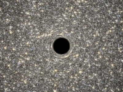
In hindsight, it seems prophetic that the title of a Nature paper published on 1 March 1974 ended with a question mark: “Black hole explosions?” Stephen Hawking’s landmark idea about what is now known as Hawking radiation1 has just turned 50. The more physicists have tried to test his theory over the past half-century, the more questions have been raised — with profound consequences for how we view the workings of reality.
In essence, what Hawking, who died six years ago today, found is that black holes should not be truly black, because they constantly radiate a tiny amount of heat. That conclusion came from basic principles of quantum physics, which imply that even empty space is a far-from-uneventful place. Instead, space is filled with roiling quantum fields in which pairs of ‘virtual’ particles incessantly pop out of nowhere and, under normal conditions, annihilate each other almost instantaneously.
However, at an event horizon, the spherical surface that defines the boundary of a black hole, something different happens. An event horizon represents a gravitational point of no return that can be crossed only inward, and Hawking realized that there two virtual particles can become separated. One of them falls into the black hole, while the other radiates away, carrying some of the energy with it. As a result, the black hole loses a tiny bit of mass and shrinks — and shines.
Unexpected ramifications
The power of Hawking’s 1974 paper lies in how it combined basic principles from the two pillars of modern physics. The first, Albert Einstein’s general theory of relativity — in which black holes manifest themselves — links gravity to the shape of space and time, and is typically relevant only at large scales. The second, quantum physics, tends to show up in microscopic situations. The two theories seem to be mathematically incompatible, and physicists have long struggled to find ways to reconcile them. Hawking showed that the event horizon of a black hole is a rare place where both theories must play a part, with calculable consequences.
Science mourns Stephen Hawking’s death
And profoundly unsettling ones at that, as quickly became apparent. The random nature of Hawking radiation means that it carries no information whatsoever. As Hawking soon realized2, this means that black holes slowly erase any information about anything that falls in, both when the black hole originally forms and subsequently as it grows — in apparent contradiction to the laws of quantum mechanics, which say that information can never be destroyed. This conundrum became known as the black-hole information paradox.
It has since turned out that black holes should not be the only things that produce Hawking radiation. Any observer accelerating through space could, in principle, pick up similar radiation from empty space3. And other analogues of black-hole shine abound in nature. For example, physicists have shown that in a moving medium, sound waves trying to move upstream seem to behave just as Hawking predicted. Some researchers hope that these experiments could provide hints as to how to solve the paradox.
A scientific wager
In the 1990s, the black-hole information paradox became the subject of a celebrated bet. Hawking, together with Kip Thorne at the California Institute of Technology (Caltech) in Pasadena, proposed that quantum mechanics would ultimately need to be amended to take Hawking radiation into account. Another Caltech theoretical physicist, John Preskill, maintained that information would be found to somehow be preserved, and that quantum mechanics would be saved.
But in 1997, theoretical physicist Juan Maldacena, who is now at the Institute for Advanced Study in Princeton , New Jersey, came up with an idea that indicated Hawking and Thorne might be wrong4. His paper now has more than 24,000 citations, even more than the 7,000 or so times Hawking’s paper has been cited. Maldacena suggested that the Universe — including the black holes it contains — is a type of hologram, a higher-dimensional projection of events that occur on a flat surface. Everything that happens on the flat world can be described by pure quantum mechanics, and so preserves information.
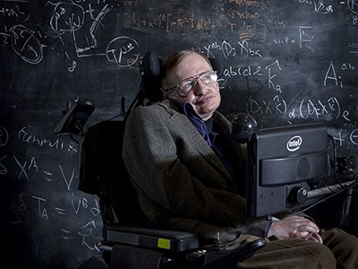
Stephen Hawking worked on the black hole information paradox throughout his life.Credit: Santi Visalli/Getty
At face value, Maldacena’s theory doesn’t fully apply to the type of Universe that we inhabit. Moreover, it did not explain how information could escape destruction in a black hole — only that it should, somehow. “We don’t have a concrete grasp of the mechanism,” says Preskill. Physicists, including Hawking, have proposed countless escape mechanisms, none of which has been completely convincing, according to Preskill. “Here it is, 50 years after that great paper, and we’re still puzzled,” he says. (Maldacena’s ideas were enough to change Hawking’s mind, however, and he conceded the bet in 2004.)
A quantum conundrum
Attempts to solve the information paradox have grown into a thriving industry. One of the ideas that has gained traction is that each particle that falls into a black hole is linked to one that stays outside through quantum entanglement — the ability of objects to share a single quantum state even when far apart. This connection could manifest itself in the geometry of space-time as a ‘wormhole’ joining the inside of the event horizon with the outside.
Entanglement is also one of the crucial features that make quantum computers potentially more powerful than classical ones. Moreover, in the past decade, the link between black holes and information theory has become only stronger, as Preskill and others have investigated similarities between what happens in holographic projections and the types of error-correction algorithm developed for quantum computers. Error correction is a way of storing redundant information that enables a computer — whether classical or quantum — to restore corrupted bits of information. Some researchers see quantum computation theory as the key to solving Hawking’s paradox. When creating a black hole, the Universe could be similarly storing several versions of its information — some inside the event horizon, some outside — so that the destruction of the black hole does not erase any history.
Hawking’s latest black-hole paper splits physicists
But other researchers think that the full resolution of the information paradox might have to wait until another big problem is solved — that of reconciling gravity with quantum physics. Hawking continued working on the problem almost up until his death, but with no clear outcome.
As for the title of Hawking’s paper, seeing actual black-hole explosions is a possibility that astronomers take seriously. Large black holes act like very cold bodies, but smaller ones are hotter, which makes them shrink faster; and the particles they shed should become more and more energetic, reaching a culmination when the black hole disappears. Hawking showed that ‘ordinary’ stellar-mass black holes, which form when massive stars collapse in on themselves at the end of their lives, take many times longer than the age of the Universe to get to this point. But, in principle, black holes with a range of smaller masses could have formed from random fluctuations in the density of matter during the first moments after the Big Bang. If a primordial black hole of the right mass were to fizzle into non-existence somewhere near the Solar System, it could be picked up by neutrino and γ-ray observatories.
Astronomers have not seen any black holes explode so far, but they are still on the lookout5. Such an observation would have certainly earned Hawking the Nobel Prize that eluded him all his life. As it is, the questions produced by his simple, inquisitive paper title look set to nourish the intersection between cosmology and physics for a good few years yet.
Trapped atomic ions are among the most advanced technologies for realizing quantum computation and quantum simulation, based on a combination of high-fidelity quantum gates1,2,3 and long coherence times7. These have been used to realize small-scale quantum algorithms and quantum error correction protocols. However, scaling the system size to support orders-of-magnitude more qubits8,9 seems highly challenging10,11,12,13. One of the primary paths to scaling is the quantum charge-coupled device (QCCD) architecture, which involves arrays of trapping zones between which ions are shuttled during algorithms13,14,15,16. However, challenges arise because of the intrinsic nature of the radio-frequency (rf) fields, which require specialized junctions for two-dimensional (2D) connectivity of different regions of the trap. Although successful demonstrations of junctions have been performed, these require dedicated large-footprint regions of the chip that limit trap density17,18,19,20,21. This adds to several other undesirable features of the rf drive that make micro-trap arrays difficult to operate6, including substantial power dissipation due to the currents flowing in the electrodes, and the need to co-align the rf and static potentials of the trap to minimize micromotion, which affects gate operations22,23. Power dissipation is likely to be a very severe constraint in trap arrays of more than 100 sites5,23.
An alternative to rf electric fields for radial confinement is to use a Penning trap in which only static electric and magnetic fields are used, which is an extremely attractive feature for scaling because of the lack of power dissipation and geometrical restrictions on the placement of ions23,24. Penning traps are a well-established tool for precision spectroscopy with small numbers of ions25,26,27,28, whereas quantum simulations and quantum control have been demonstrated in crystals of more than 100 ions29,30,31. However, the single trap site used in these approaches does not provide the flexibility and scalability necessary for large-scale quantum computing.
Invoking the idea of the QCCD architecture, the Penning QCCD can be envisioned as a scalable approach, in which a micro-fabricated electrode structure enables the trapping of ions at many individual trapping sites, which can be actively reconfigured during the algorithm by changing the electric potential. Beyond the static arrays considered in previous work23,32, here we conceptualize that ions in separated sites are brought close to each other to use the Coulomb interaction for two-qubit gate protocols implemented through applied laser or microwave fields33,34, before being transported to additional locations for further operations. The main advantage of this approach is that the transport of ions can be performed in three dimensions almost arbitrarily without the need for specialized junctions, enabling flexible and deterministic reconfiguration of the array with low spatial overhead.
In this study, we demonstrate the fundamental building block of such an array by trapping a single ion in a cryogenic micro-fabricated surface-electrode Penning trap. We demonstrate quantum control of its spin and motional degrees of freedom and measure a heating rate lower than in any comparably sized rf trap. We use this system to demonstrate flexible 2D transport of ions above the electrode plane with negligible heating of the motional state. This provides a key ingredient for scaling based on the Penning ion-trap QCCD architecture.
The experimental setup involves a single beryllium (9Be+) ion confined using a static quadrupolar electric potential generated by applying voltages to the electrodes of a surface-electrode trap with geometry shown in Fig. 1a–c. We use a radially symmetric potential \(V(x,y,z)=m{\omega }_{z}^{2}({z}^{2}-({x}^{2}+{y}^{2})/2)/(2e)\), centred at a position 152 μm above the chip surface. Here, m is the mass of the ion, ωz is the axial frequency and e is the elementary charge. The trap is embedded in a homogeneous magnetic field aligned along the z-axis with a magnitude of B≃ 3 T, supplied by a superconducting magnet. The trap assembly is placed in a cryogenic, ultrahigh vacuum chamber that fits inside the magnet bore, with the aim of reducing background-gas collisions and motional heating. Using a laser at 235 nm, we load the trap by resonance-enhanced multiphoton ionization of neutral atoms produced from either a resistively heated oven or an ablation source35. We regularly trap single ions for more than a day, with the primary loss mechanism being related to user interference. Further details about the apparatus can be found in the Methods.
Fig. 1: Surface-electrode Penning trap.
a, Schematic showing the middle section of the micro-fabricated surface-electrode trap. The trap chip is embedded in a uniform magnetic field along the z axis, and the application of d.c. voltages on the electrodes leads to 3D confinement of the ion at a height h≃ 152 μm above the surface. Electrodes labelled ‘d.c. + rf’ are used for coupling the radial modes during Doppler cooling. b, Micrographic image of the trap chip, with an overlay of the direction of the laser beams (all near 313 nm) and microwave radiation (near ω0≃ 2π × 83.2 GHz) required for manipulating the spin and motion of the ion. All laser beams run parallel to the surface of the trap and are switched on or off using acousto-optic modulators, whereas microwave radiation is delivered to the ion by a horn antenna close to the chip. Scale bar, 100 μm. c, Epicyclic motion of the ion in the radial plane (x–y) resulting from the sum of the two circular eigenmodes, the cyclotron and the magnetron modes. d, Electronic structure of the 9Be+ ion, with the relevant transitions used for coherent and incoherent operations on the ion. Only the levels with nuclear spin mI = +3/2 are shown. The virtual level (dashed line) used for Raman excitation is detuned ΔR≃ +2π × 150 GHz from the 2p 2P3/2 |mI = +3/2, mJ = +3/2⟩ state.
The three-dimensional (3D) motion of an ion in a Penning trap can be described as a sum of three harmonic eigenmodes. The axial motion along z is a simple harmonic oscillator with frequency ωz. The radial motion is composed of modified-cyclotron (ω+) and magnetron (ω−) components, with frequencies ω± = ωc/2 ± Ω, where \(\varOmega =\sqrt{{\omega }_{{\rm{c}}}^{2}-2{\omega }_{z}^{2}}/2\) (ref. 36) and ωc = eB/m≃ 2π × 5.12 MHz is the bare cyclotron frequency. Voltage control over the d.c. electrodes of the trap enables the axial frequency to be set to any value up to the stability limit, ωz ≤ ωc/\(\sqrt{2}\)≃ 2π × 3.62 MHz. This corresponds to a range 0 ≤ ω− ≤ 2π × 2.56 MHz and 2π × 2.56 MHz ≤ ω+ ≤ 2π × 5.12 MHz for the magnetron and modified-cyclotron modes, respectively. Doppler cooling of the magnetron mode, which has a negative total energy, is achieved using a weak axialization rf quadrupolar electric field (less than 60 mV peak-to-peak voltage on the electrodes) at the bare cyclotron frequency, which resonantly couples the magnetron and modified-cyclotron motions37,38. For the wiring configuration used in this work, the null of the rf field is produced at a height h≃ 152 μm above the electrode plane. Aligning the null of the d.c. (trapping) field to the rf null is beneficial because it reduces the driven radial motion at the axialization frequency; nevertheless, we find that Doppler cooling works with a relative displacement of tens of micrometres between the d.c. and rf nulls, albeit with lower efficiency. The rf field is required only during Doppler cooling, and not, for instance, during coherent operations on the spin or motion of the ion. All measurements in this work are taken at an axial frequency ωz≃ 2π × 2.5 MHz, unless stated otherwise. The corresponding radial frequencies are ω+≃ 2π × 4.41 MHz and ω−≃ 2π × 0.71 MHz.
Figure 1d shows the electronic structure of the beryllium ion along with the transitions relevant to this work. We use an electron spin qubit (consisting of the \(|\uparrow \rangle \equiv |{m}_{{\rm{I}}}=+\,3/2,{m}_{{\rm{J}}}=+\,1/2\rangle \) and \(|\downarrow \rangle \equiv |{m}_{{\rm{I}}}\,=+\,3/2,{m}_{{\rm{J}}}=-\,1/2\rangle \) eigenstates within the 2s 2S1/2 ground-state manifold), which in the high field is almost decoupled from the nuclear spin. The qubit frequency is ω0≃ 2π × 83.2 GHz. Doppler cooling is performed using the detection laser red-detuned from the (bright) |↑⟩ ↔ 2p 2P3/2 |mI = +3/2, mJ = +3/2⟩ cycling transition, whereas an additional repump laser optically pumps population from the (dark) |↓⟩ level to the higher energy |↑⟩ level through the fast-decaying 2p 2P3/2 |mI = +3/2, mJ = +1/2⟩ excited state. State-dependent fluorescence with the detection laser allows for discrimination between the two qubit states based on photon counts collected on a photomultiplier tube using an imaging system that uses a 0.55 NA Schwarzschild objective. The fluorescence can also be sent to an electron-multiplying CCD (EMCCD) camera.
Coherent operations on the spin and motional degrees of freedom of the ion are performed either using stimulated Raman transitions with a pair of lasers tuned to 150 GHz above the 2p 2P3/2 |mI = +3/2, mJ = +3/2⟩ state or using a microwave field. The former requires the use of two 313 nm lasers phase-locked at the qubit frequency, which we achieve using the method outlined in ref. 39. By choosing different orientations of Raman laser paths, we can address the radial or axial motions, or implement single-qubit rotations using a co-propagating Raman beam pair.
The qubit transition has a sensitivity of 28 GHz T−1 to the magnetic field, meaning the phase-coherence of our qubit is susceptible to temporal fluctuations or spatial gradients of the field across the extent of the motion of the ion. Using Ramsey spectroscopy, we measure a coherence time of 1.9(2) ms with the Raman beams. Similar values are measured with the microwave field, indicating that laser phase noise from beam path fluctuations or imperfect phase-locking does not significantly contribute to dephasing. The nature of the noise seems to be slow on the timescale (about 1 ms to 10 ms) of a single experimental shot consisting of cooling, probing and detection, and the fringe contrast decay follows a Gaussian curve. We note that the coherence is reduced if vibrations induced by the cryocoolers used to cool the magnet and the vacuum apparatus are not well decoupled from the experimental setup. Further characterization of the magnetic field noise is performed by applying different orders of the Uhrig dynamical decoupling sequence40,41, with the resulting extracted coherence time from the measurements being 3.2(1) ms, 5.8(3) ms and 8.0(7) ms for orders 1, 3 and 5, respectively. Data on spin-dephasing are presented in Extended Data Fig. 1.
A combination of the Doppler cooling and repump lasers prepares the ion in the |↑⟩ electronic state and a thermal distribution of motional Fock states. After Doppler cooling using the axialization technique, we measure mean occupations of \(\{{\bar{n}}_{+},{\bar{n}}_{-},{\bar{n}}_{z}\}=\{6.7(4),9.9(6),4.4(1)\}\) using sideband spectroscopy on the first four red and blue sidebands38. Pulses of continuous sideband cooling31,38 are subsequently performed by alternatively driving the first and third blue sidebands of a positive energy motional mode and red sidebands of a negative energy motional mode while simultaneously repumping the spin state to the bright state. The 3D ground state can be prepared by applying this sequence for each of the three modes in succession. The use of the third sideband is motivated by the high Lamb–Dicke parameters of approximately 0.4 in our system42,43. After a total time of 60 ms of cooling, we probe the temperature using sideband spectroscopy on the first blue and red sidebands44. Assuming thermal distributions, we measure \(\{{\bar{n}}_{+},{\bar{n}}_{-},{\bar{n}}_{z}\}=\{0.05(1),0.03(2),0.007(3)\}\). We have achieved similar performance of the ground-state cooling at all trap frequencies probed to date. The long duration of the sideband cooling sequence stems from the large (estimated as 80 μm) Gaussian beam radius of the Raman beams each with power in the range of 2 mW to 6 mW, leading to a Rabi frequency Ω0≃ 2π × 8 kHz, which corresponds to π times of approximately 62 μs, 145 μs and 2,000 μs for the ground-state carrier, first and third sidebands, respectively, at ωz = 2π × 2.5 MHz.
Trapped-ion quantum computing uses the collective motion of the ions for multi-qubit gates and thus requires the motional degree of freedom to retain coherence over the timescale of the operation33,45. A contribution to decoherence comes from motional heating due to fluctuations in the electric field at frequencies close to the oscillation frequencies of the ion. We measure this by inserting a variable-length delay twait between the end of sideband cooling and the temperature probe. As shown in Fig. 2, we observe motional heating rates \(\{{\dot{\bar{n}}}_{+},{\dot{\bar{n}}}_{-},{\dot{\bar{n}}}_{z}\}=\{0.49(5)\,{{\rm{s}}}^{-1},3.8(1)\,{{\rm{s}}}^{-1},0.088(9)\,{{\rm{s}}}^{-1}\}\). The corresponding electric-field spectral noise density for the axial mode, \({S}_{{\rm{E}}}=4\hbar m{\omega }_{z}{\dot{\bar{n}}}_{z}/{e}^{2}=3.4(3)\times {10}^{-16}\,{{\rm{V}}}^{2}{{\rm{m}}}^{-2}{{\rm{Hz}}}^{-1}\), is lower than any comparable measurement in a trap of similar size46,47. As detailed in the Methods, we can trap ions in our setup with the trap electrodes detached from any external supply voltage except during Doppler cooling, which requires the axialization signal to pass to the trap. Using this method, we measure heating rates \({\dot{\bar{n}}}_{z}=0.10(1)\,{{\rm{s}}}^{-1}\) and \({\dot{\bar{n}}}_{+}=0.58(2)\,{{\rm{s}}}^{-1}\) for the axial and cyclotron modes, respectively, whereas the rate for the lower-frequency magnetron mode drops to \({\dot{\bar{n}}}_{-}=1.8(3)\,{{\rm{s}}}^{-1}\). This reduction suggests that external electrical noise contributes to the higher magnetron heating rate in the earlier measurements.
Fig. 2: Motional coherence.
a, Bright-state population P↑ measured after applying the first red or blue axial sideband probe-pulse to the sideband-cooled ion. As the bright state |↑⟩ has a higher energy than the dark state |↓⟩, the blue sideband cannot be driven when the ion is in the ground state of the axial mode. b, Average phonon number \(\bar{n}\) calculated using the sideband-ratio method44 for all three modes as a function of increasing twait. The purple and orange points indicate data taken with the trap connected and detached, respectively. The heating rates are extracted from the slopes of the linear fits. c, Motional dephasing of the axial mode observed by Ramsey spectroscopy. The purple points indicate data taken with an echo pulse in the sequence. The orange points indicate data taken with an echo pulse, in which, additionally, the trap was detached between Doppler cooling and the detection pulse. Whereas the dataset with the voltage sources detached is taken at ωz≃ 2π × 2.5 MHz, the two data series with the trap attached are taken at an axial mode frequency ωz≃ 2π × 3.1 MHz. The dashed lines show the 1/e line normalized to the Gaussian fits. All error bars indicate the standard error.
Motional-state dephasing was measured using Ramsey spectroscopy, involving setting up a superposition |↑⟩ (|0⟩z + |1⟩z)/\(\sqrt{2}\) of the first two Fock states of the axial mode (here ωz≃ 2π × 3.1 MHz) using a combination of carrier and sideband pulses48. Following a variable wait time, we reverse the preparation sequence with a shifted phase. The resulting decay of the Ramsey contrast shown in Fig. 2c is much faster than what would be expected from the heating rate. The decay is roughly Gaussian in form with a 1/e coherence time of 66(5) ms. Inserting an echo pulse in the Ramsey sequence extends the coherence time to 240(20) ms, which indicates low-frequency noise components dominating the bare Ramsey coherence. Further improvement of the echo coherence time to 440(50) ms is observed when the trap electrodes are detached from external voltage sources between the conclusion of Doppler cooling and the start of the detection pulse, in which again the axialization signal is beneficial. The data with the voltage sources detached are taken at ωz≃ 2π × 2.5 MHz.
An important component of the QCCD architecture14 is ion transport. We demonstrate that the Penning trap approach enables us to perform this flexibly in two dimensions by adiabatically transporting a single ion, and observing it at the new location. The ion is first Doppler-cooled at the original location, and then transported in 4 ms to a second desired location along a direct trajectory. We then perform a 500-μs detection pulse without applying axialization and collect the ion fluorescence on an EMCCD camera. The exposure of the camera is limited to the time window defined by the detection pulse. The lack of axialization is important when the ion is sufficiently far from the rf null to minimize radial excitation due to micromotion and subsequently produce enough fluorescence during the detection window. The ion is then returned to the initial location. Figure 3 shows a result in which we have drawn the first letters of the ETH Zürich logo. The image quality and maximum canvas size are only limited by the point-spread function and field of view of our imaging system, as well as the spatial extent of the detection laser beam, and not by any property of the transport. Reliable transport to a set location and back has been performed up to 250 μm. By probing ion temperatures after transport using sideband thermometry (Extended Data Fig. 2), we have observed no evidence of motional excitation from transport compared with the natural heating expected over the duration of the transport. This contrasts with earlier non-adiabatic radial transport of ensembles of ions in Penning traps, in which a good fraction of the ions were lost in each transport49.
Fig. 3: Demonstration of 2D transport.
A single ion is transported adiabatically in the x–z plane (normal to the imaging optical axis). The ion is illuminated for 500 μs at a total of 58 positions, here defined by the ETH Zürich logo (see inset for reference image). The red circle indicates the initial position in which the ion is Doppler-cooled. The ion is moved across a region spanning approximately 40 μm and 75 μm along the x (radial) and z (axial) directions, respectively. The sequence is repeated 172 times to accumulate the image.
This work marks a starting point for quantum computing and simulation in micro-scale Penning trap 2D arrays. The next main step is to operate with multiple sites of such an array, which will require optimization of the loading while keeping the ions trapped in shallow potentials. This can be accomplished in the current trap with the appropriate wiring, but notable advantages could be gained by using a trap with a loading region and shuttling ions into the micro-trap region. Multi-qubit gates could then be implemented following the standard methods demonstrated in rf traps23,34. Increased spin-coherence times could be achieved through improvements to the mechanical stability of the magnet, or in the longer term through the use of decoherence-free subspaces, which were considered in the original QCCD proposals14,50,51. For scaling to large numbers of sites, it is likely that scalable approaches to light delivery will be required, which might necessitate switching to an ion species that is more amenable to integrated optics52,53,54,55. The use of advanced standard fabrication methods such as CMOS56,57 is facilitated, compared with rf traps, by the lack of high-voltage rf signals. Compatibility with these technologies demands an evaluation of how close to the surface ions could be operated for quantum computing and will require in-depth studies of heating—here an obvious next step is to sample electric field noise as a function of ion-electrode distance47. Unlike in rf traps, 3D scans of electric field noise are possible in any Penning trap because of the flexibility of confinement to the uniform magnetic field. This flexibility of ion placement has advantages in many areas of ion-trap physics, for instance, in placing ions in anti-nodes of optical cavities58, or sampling field noise from surfaces of interest59,60. We, therefore, expect that our work will open previously unknown avenues in sensing, computation, simulation and networking, enabling ion-trap physics to break out beyond its current constraints.